
APOGEE Stellar Parameter and Abundance Determination
One main objective of the APOGEE survey is to extract the chemical abundances of several elements for the entire stellar sample. To determine these element abundances, the stellar atmospheric parameters — effective temperature, surface gravity, overall metallicity, and microturbulent velocity — must be known a priori. The APOGEE Stellar Parameters and Chemical Abundances Pipeline (ASPCAP) employs a two-step process to extract abundances: first, determination of the atmospheric parameters by fitting the entire APOGEE spectrum, and second, use of these parameters to fit various small regions of the spectrum dominated by spectral features associated with a particular element in order to derive the individual element abundance ([X/H] or [X/M], see below).
APOGEE uncertainties
APOGEE reports uncertainties as standard deviations.
This is in contrast to the optical spectral pipelines (such as the Optical Spectroscopy Pipeline or the SEGUE Stellar Parameter Pipeline), which typically report uncertainties as inverse variances.
The wavelength region covered by the APOGEE spectra includes a vast number of atomic transitions of many elements, but molecular features, in particular, from CN, CO, and OH can be very prominent, especially in cooler stars that comprise the bulk of the survey sample. A global fit needs to include the possibility of variations in elemental abundance ratios that have a significant effect in the equation of state (e.g. through CO formation or contributing free electrons) or the opacity. For this reason, the stellar parameters portion of the ASPCAP pipeline allows for variations in seven parameters: effective temperature, surface gravity, microturbulence, overall metal abundance [M/H] , relative α-element abundance [α /M] (defined as O, Mg, Si, S, Ca, and Ti changing with solar proportions in lockstep), carbon [C/M], and nitrogen [N/M] abundances.
On this page, we describe the basic operation of ASPCAP. Please consult Garcia-Perez et al. (2015) for further details.
For a discussion of the quality of the derived parameters, and important things to know about using them, all users of ASPCAP results should read Using APOGEE stellar parameters. For a discussion of the quality of the individual elemental abundances, and important things to know about using them, all users of ASPCAP results should read Using APOGEE chemical abundances.
The APOGEE abundance scale
The abundance of each individual element X heavier than helium, is defined as
[X/H] = log10 (nX/nH) - log10(nX/nH)☉
where nX and nH are respectively the number of nuclei of element X and hydrogen, per unit volume in the stellar photosphere. We define [M/H] as an overall scaling of metal abundances with a solar abundance ratio pattern, and [X/M] as the deviation of element X from the solar abundance pattern:
[X/M] = [X/H] - [M/H]☉
Once the stellar parameters have been determined, abundances for individual elements are derived individually, by fitting the spectrum in limited spectral windows that contain features of the desired element (see the section on abundances below).
In DR12, we provide the best fitting values of the global stellar parameters as well as individual elemental abundances for Al, Ca, C, Fe, K, Mg, Mn, Na, Ni, N, O, Si, S, Ti, and V. The raw measurements from the fits to the spectral grid are calibrated, predominantly using observations of stellar clusters. For more details, see the section on calibration below.
Some caveats apply. The abundances are NOT truly differential to the Sun. Solar abundances are adopted from Asplund et al. (2005), and used for computing model atmospheres (see Mészáros et al. 2012) and synthetic spectral grids. The line list used for spectral synthesis includes, in addition to laboratory and theoretical transition probabilities and damping constants, modifications to match the solar spectrum and that of the red giant Arcturus. Please consult Shetrone et al. (2015) for further details.
Therefore, the abundances are not strictly differential to those of the Sun, but APOGEE DR12 includes a spectrum of the Sun observed through reflected light on the asteroid Vesta. That allows us to check zero-point offsets from a truly differential approach for the Sun, and these offsets are fairly small, with a mean under 0.02 dex and a standard deviation under 0.1 dex.
APOGEE Stellar Parameters and Chemical Abundances Pipeline (ASPCAP)
ASPCAP Components
- Large grids of synthetic spectra are computed for the APOGEE wavelength region, using a custom linelist derived for this portion of the spectrum. The grids cover the full expected range of the seven parameters mentioned above: Teff, log g, vmicro, [M/H], [α/M], [C/M], and [N/M]. The synthetic spectra are “pseudo-continuum normalized” by iterative fitting by least squares and sigma-clipping a polynomial to the fluxes. The sigma clipping has asymmetric limits for rejection, rejecting more vigorously lower points, with the goal of pushing the polynomial to the upper envelope of the spectrum.
- Combined APOGEE spectra are pseudo-continuum normalized to remove variations of spectral shape arising from interstellar reddenning, errors in relative fluxing, and atmospheric absorption. This normalization is done the same way as for the synthetic spectra, so that they can be directly compared (the true continuum level is hard to determine from the observed spectra).
- An independent code (FERRE — see Allende Prieto et al. 2006) searches for the best matching synthetic spectrum for each star via χ2 minimization technique, allowing for interpolation in the synthetic spectra grid.
- From the results of the different synthetic grids, the best-fit synthetic spectrum is identified for each object, and the best-fitting results for all of the stars are compiled.
- Using the best-fit parameters, small windows around features of specific individual elements are fit to derive the elemental abundances.
- Internal calibration relations are applied that make small temperature-dependent corrections to the abundances; these were derived by looking at abundances as a function of temperature within (mostly metal-rich, open) clusters, under the assumptions that these clusters have homogenous abundances. Using results from the derived parameters for objects of known parameters, some external calibration relations have been derived, and these relations are applied to some of the derived parameters. In addition, this stage sets a series of data quality flags for the stellar parameter and abundances results.
This procedure works only as well as the synthetic spectra match the observed data, and to the degree that the observed data contain parameter and abundance information. At cooler temperatures (T<4000K) the model spectra do not match as well, so parameters and abundances there are currently less certain. At warmer temperatures (T>5500 K), spectral features of some elements become very weak, so their measurement is significantly less certain.
Stellar Spectral Libraries (pre-computed)
Grids of normalized stellar synthetic spectra are computed with the spectral synthesis code ASSET (Koesterke et al. 2008; Koesterke 2009), using ATLAS9 (or MARCS) model atmospheres described by Mészáros et al. 2012, and a line list for the APOGEE wavelength region compiled from the literature and tuned to match the spectrum of the Sun (see Shetrone et al., in preparation). The model atmospheres and the synthetic spectra adopt solar abundances by Asplund et al. 2005, but with varying metallicities, carbon, and α-element abundances. Variations in nitrogen abundances are also considered, but only at the synthesis stage (not in the model atmospheres).
The synthetic spectra are smoothed using a line spread function (LSF) measured from APOGEE sky spectra. However, the LSF varies with wavelength and location in the frame. For the current analysis, we have averaged the LSFs from five fibers across the frame, preserving the wavelength variation, and analyzed all spectra using the library smoothed with this average LSF. Initial tests suggest that the assumption of a constant LSF does not change the derived parameters by much (see Garcia-Perez et al 2015), although future work may incorporate the LSF variations. In addition to the LSF smoothing, we have also including smoothing to account for macroturbulent velocities; we implement this with Gaussian smoothing with FWHM corresponding to 6 km/s.
After smoothing, the library spectra are interpolated onto the same wavelength scale as the combined APOGEE spectra, and pseudocontinuum normalized.
Ideally we would store the entire grid of stellar spectra in memory to allow for efficient computation comparison of our observed normalized data to the spectrum match each grid point. However, the multi-dimensional synthetic spectrum library is too large to store simultaneously in the memory of a typical computer. For this reason, the flux arrays are compressed using Principal Component Analysis, and the full parameter space is split into different grids that cover different temperature regimes. For DR12 we use two grids: the GK grid which covers 3500-6000 K, and the F grid which covers 5500-8000 K.
In general, seven parameters are required to adequately describe the spectra: effective temperature, surface gravity, microturbulence, metal abundance (all elements heavier than He), α element (O, Mg, Si, S, Ca, and Ti) relative abundance, carbon relative abundance, and nitrogen relative abundance. However, for hotter stars, there may not be sufficient information to independently determine all of these parameters.
Full fits in seven dimensions are computationally expensive. To reduce the required computing resources, we did 7D fits only for a calibration subsample, and from this, derived a relation between the microturbulence and surface gravity:
Vmicro=2.48-0.32*log g
We then used this relation to do 6D fits for the entire APOGEE sample.
The following table summarizes the synthetic grids:
| Class | Dimensions | T | log g | [M/H] | [C/M] | [N/M] | [α/M] |
|---|---|---|---|---|---|---|---|
| GK | 6 | 3500 to 6000 | 0 to 5 | -2.5 to 0.5 | -1 to 1 | -1 to 1 | -1 to 1 |
| step: 250 | step: 0.5 | step: 0.5 | step: 0.25 | step: 0.5 | step: 0.25 | ||
| F | 6 | 5500 to 8000 | 1 to 5 | -2.5 to 0.5 | -1 to 1 | -1 to 1 | -1 to 1 |
| step:250 | step: 0.5 | step: 0.5 | step: 0.25 | step: 0.55 | step: 0.25 |
ASPCAP Pre-processing
The comparison of observations with the library requires the pre-processing of the combined APOGEE spectra, which is carried out by an IDL wrapper, and consists of masking out bad pixels and normalizing the spectra.
- Since FERRE minimizes χ2, realistic estimates of flux uncertainties are critical, and any bad data must be masked. Pixels flagged as bad (saturated, cosmic ray, etc) in the data-reduction process and pixels around the sky emission lines are ignored for continuum normalization, and in the χ2 minimization. To account for small systematic errors in spectral calibration, we set a minimum error of 0.5 percent for all pixels.
- To normalize the spectra, the spectral regions covered by each of the three chips used in the APOGEE spectrograph are considered separately. In each region, a sigma-clipping algorithm is used to fit a polynomial to the upper envelope of the spectrum. In order to allow a meaningful comparison to the library of synthetic spectra, an identical normalization is performed on the library, using the same spectral regions with the same sigma-clipping and polynomial form. We emphasize that this normalization is not a normalization to the true continuum, because, especially for metal-rich stars, the upper envelope of the data may still not be at the true continuum level. Thus, we do not calculate abundances from equivalent widths from these “pseudo-continuum” normalized spectra, but rather comparing to models that have had the same normalization procedure applied.
Determination of stellar parameters (FERRE)
Stellar parameters and the relative abundances of C, N and α-elements are determined by the FORTRAN90 code FERRE, which compares the observations with the grid of pre-computed synthetic spectra. The code uses a χ2 criterion as the merit function, and searches for the best matching synthetic spectrum using the Nelder-Mead algorithm (Nelder and Mead 1965). The search is run 12 times starting from different locations: the center of the grid for [C/M], [N/M] and [α/M], and at two different places symmetrically located from the grid center for [M/H] and log g, and at three for Teff. Interpolation within the grid of synthetic spectra is accomplished using cubic Bezier interpolation. The code returns the best matching spectrum, the parameters associated with that spectrum (stellar parameters and [C/M], [N/M] and [α/M] abundance ratios), the covariance matrix of these parameters, and the χ2 value for the best-matching spectrum.
Abundance determination
The abundance derivation takes place after the atmospheric parameters (Teff, log g, vmicro, [M/H], [α/M], [C/M], and [N/M]) have been simultaneously determined from the APOGEE spectra. A second call to the optimization program (FERRE) is performed for the abundance determination. For these fits, the same library of synthetic spectra is used, but with two main changes:
- Abundances of individual alpha elements (O, Mg, Si, S, Ca, and Ti) are derived by varying the [α/M] dimension of the grid, the abundance of carbon and nitrogen by varying the [C/M] and [N/M] dimensions, and the abundances of all other elements by varying the [M/H] dimension. All other atmospheric parameters are held at the values previous determined.
- The weights for the chi-square calculations are now changed so that only we only consider spectral features that are primarily sensitive to the element we are interested in. The assumption here is that, within the defined windows (see below), the abundance of the desired element dominates over variations from other elements contained in the same grid dimension.
Therefore, we are not really changing the element of interest only, but the element of interest and others: all alpha elements as a block when fitting an alpha element, or all metals when changing a non-alpha element. This approach works well when the abundance we derive is not very different from the group it belongs to (either just the alpha elements, or all metals).
Transitions used (weight determination)
Deriving the relevant weights for each element is basically equivalent to deciding which transitions and which parts of the line profiles are to be used for each element.
This is accomplished by using first a algorithm that evaluates the derivatives of the model fluxes with respect to each elemental abundance for a star like Arcturus (Teff=4300 K, logg=1.7, [Fe/H]=-0.5). Frequencies (wavelengths) at which the module of the derivative for the element of interest is large are given a high weight, with a negative contribution when the module of the derivatives are large for any other element. Weights are adjusted with a multiplicative factor that takes into account how well the model spectrum for Arcturus reproduces an actual observation of this star. A second multiplicative factor takes into account how well APOGEE spectra are reproduced by the model fluxes, using the median residuals at each frequency based on fitting the entire APOGEE sample.
Finally, the list of weights are cleaned-up by hand, based on visual inspection of the fittings for each element in a set of reference stars by Smith et al. (2013).
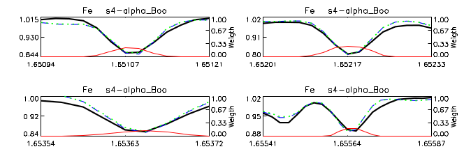
The number of transitions/features used for each element varies from element to element: there are 45 for C (C I, but mainly CO and CN), 77 for N (CN), 50 for O (OH), 2 for Na (Na I), 4 for Mg (Mg I), 2 for Al (Al I), 10 for Si (Si I), 3 for S (S I), 1 for K (K I), 3 for Ca (Ca I), 5 for Ti (Ti I and Ti II), 2 for V (V I), 4 for Mn (Mn I), 61 for Fe (Fe I), and 7 for Ni (Ni I). The attached pdf file shows the fittings for the observations of Arcturus in the Hinkle et al. (1995) atlas (smoothed with a Gaussian profile to R~22,500) and this one is the equivalent for the APOGEE observation of the same star from thee APO 1m telescope (with 4 Fe I transitions illustrated in the following figure).
ASPCAP post-processing
Once FERRE has delivered results for the different temperature grids, the IDL wrapper chooses the result that produces the lowest χ2. These results (pseudo continuum, normalized observed spectra, flux errors, stellar parameters and [C/M], [N/M], [α/M] values, covariance matrix, χ2 values) along with other relevant information (e.g. 2MASS photometry, reddening, radial velocities, signal-to-noise ratios etc.) are compiled.
Calibration and Final Error Estimates of the Parameters
In addition to the raw FERRE output parameters, we also provide a calibrated set of parameters. Temperatures and surface gravities are calibrated relative to independent measurements of these quantities in a calibration subset. Abundance parameters and abundances are internally calibrated to provide homogeneous results within clusters. The metallicity parameter [M/H] is also externally calibrated based on independent metallicity determinations of clusters.
Internal calibration
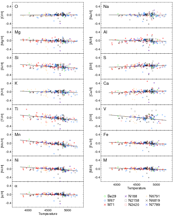
The abundance parameters ([M/H] and [α/M], as well as all of the individual element abundances are internally calibrated based on observations of stellar clusters with [Fe/H]>-1. Under the assumption that such clusters have internally homogeneous abundances, we find small systematic variations of abundance with temperature, and use these to derive internal calibration relations of the form:
[X/H] = [X/H]ASPCAP + S (Teff,ASPCAP-4500 )
to provide internally calibrated abundances. We do not do this for carbon and nitrogen, which are known to have varying abundances due to mixing along the giant branch.
The internal calibration is derived almost entirely from observations of giants, so we do know not to what extent it might apply to stars with higher surface gravity. As a result, we do not provide calibrated abundances for such stars. Also, even among giants, the calibration sample is restricted in temperature range from around 3800K to 5250K; for sample stars outside this range, we apply the correction at the edge of the range (i.e., we don’t extrapolate the relation), and set a bit (CALRANGE_WARN) in the abundance flags.
External calibration
The data used to derive the calibration relations and the derivation of the relations themselves are described in Holtzman et al. (2015). The calibrations are summarized here:
- Temperatures have been calibrated to photometric temperatures using the González Hernández and Bonifacio (2009) IRFM scale.
Teff = TeffASPCAP + 88 - Corrections for the surface gravities were estimated from a set of stars observed in the Kepler field, for which asteroseismic analysis yields highly accurate surface gravities. There is an apparent offset in the derived calibration from red giant and red clump stars that is currently not well-understood; the current calibration is derived from the red giant sample:
log g = log gASPCAP + 0.14 log g ASPCAP -0.588
Because of the discrepancy between red giants and red clump stars, there is a significant concern about the possibility of systematic issues with the surface gravities. - The parameter-level metallicity results [M/H] have been externally calibrated using a sample of well studied clusters covering a wide range of metallicities (M/H]=-2.35–+0.47) against their overall published spectroscopic metallicities.
[M/H] ~ [M/H]ASPCAP +0.026 + 0.255 [M/H]ASPCAP +0.062 [M/H]ASPCAP>2 - Because of the challenge of finding homogeneous reference abundances for individual elements, the individual [X/H] abundances have not had any external calibration applied to them, including [Fe/H]. As a result, the calibrated [Fe/H] will not match the calibrated [M/H], even though the raw ASPCAP values match closely.
- Empirical parameter and abundance uncertainties have been estimated based on scatter observed within clusters. See the abundance uncertainty section of the Using Abundances page for additional details.
Output data files
ASPCAP is generally run separate for each APOGEE field (i.e. location in the sky). The ASPCAP output for all stars in the field is stored in a single aspcapField file. Results for each individual star are stored in aspcapStar files. See the links for a full description of the data in these files, but briefly, these files are binary FITS tables that contain three separate tables: the first contains the information about the star and the derived stellar parameters, the second contains the observed and best-matching synthetic spectra, and the third contains library and wavelength information.