
Galaxy Properties from the Wisconsin Group
[Back to main galaxy properties page]
Principal Component Analysis (PCA) Method
Chen et al. (2012) model physical galaxy parameters based on a library of model spectra for which principal components (PCs) have been identified. The method is applied in the following steps.
Create library of model spectra
The two libraries of model spectra, for the bc03 and m11 configurations, are based on:
- Bruzual & Charlot (2003) stellar population synthesis models,
- Maraston & Strömbäck (2011) stellar population synthesis models,
respectively. These models are parameterized by the following characteristics.
- Star formation histories (SFHs)
- Each SFH consists of three parts: an underlying continuous model + a series of super-imposed stochastic bursts + a random probability for star formation to stop exponentially (i.e. truncation). Figure 1 shows three examples of SFHs. The top panel is a continuous model, middle panel shows a continuous model with two random bursts, a truncation can be found in the bottom panel.
-
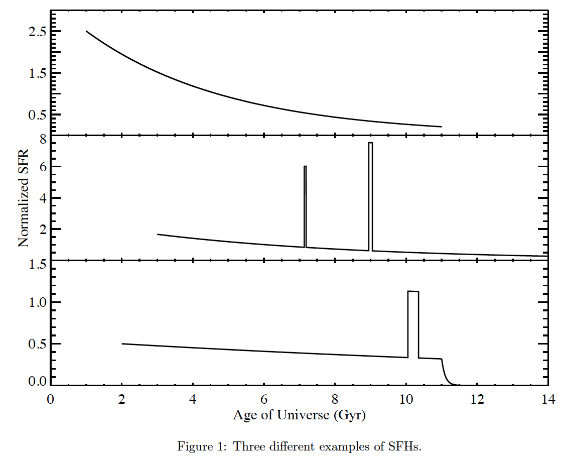
Figure 1: Three different examples of SFHs. - Metallicity
- 95% of the model galaxies in the library are distributed uniformly in metallicity from 0.2 – 2.5 Z☉; 5% of the model galaxies are distributed uniformly between 0.02 and 0.2 Z☉.
- Dust extinction
- Dust extinction is modeled using the two-component model described in Charlot & Fall (2000). The V-band optical depth has a Gaussian distribution over the range 0 < τV < 6. with a peak at 1.2 and 68% of the total probability distribution distributed over the range 0~2. This prior distribution of τV values is motivated by the observed distribution of Balmer decrements in SDSS spectra (Brinchmann et al. 2004). The fraction of the optical depth that affects stellar populations older than 0.01 Gyr is parameterized as μ, which is again modeled as a Gaussian with a peak at μ = 0.3, and a 68 percentile range of 0.1~1.
- Velocity dispersion
- Each of the model spectra is convolved to a velocity that is uniformly distributed over the range of values from 75 to 400 km/s.

Principal components (PCs) are identified from the model library
The regions around nebular emission lines are masked in the model spectra. We mask 500 km/s around the [OII]3726.03, [OII]3728.82, Hζ3889.05, [NeIII]3869.06, Hδ4101.73, Hγ4340.46, Hβ4861.33, [OIII]4959.91, and [OIII]5007.84 Å lines. Each spectrum in the masked library is normalized to its mean flux between 3700-5500 Å (this is the range we use for analysis). The mean spectrum of the masked library is calculated and subtracted from each of the model spectra.
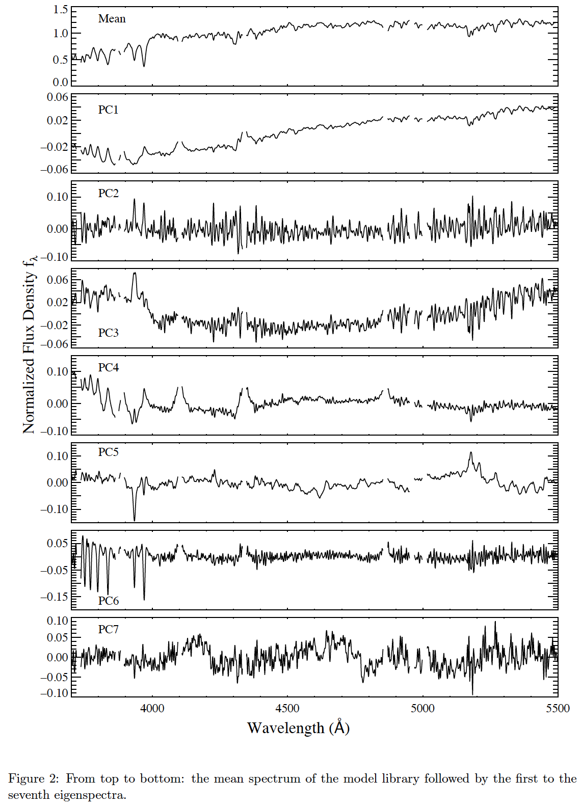
PCA code is run on the “residual” spectra. Figure 2 presents the mean spectrum and the top seven PCs for the input model library.
Project BOSS data and models onto PCs
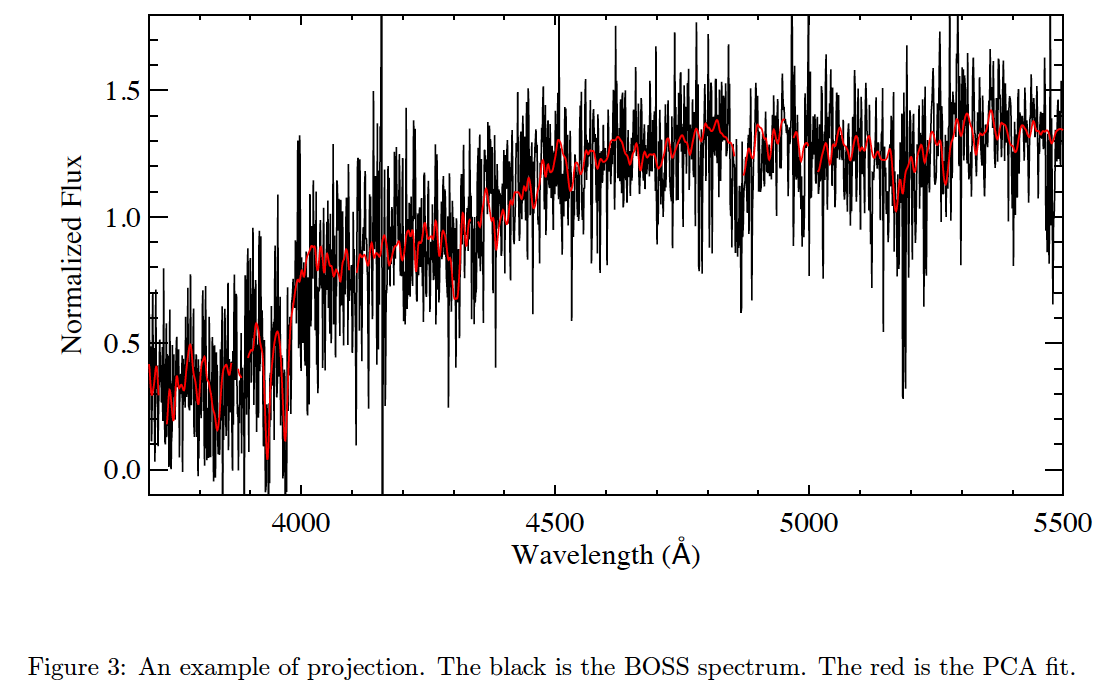
Figure 3 shows an example of projection. The black is the BOSS spectrum. The red is the PCA fit, it is a linear combination of the mean spectrum and the PCs, namely, fit = mean + C1 × PC1 + C2 × PC2 + … + C7 × PC7, where Cα (α = 1–7) are the coefficients of the projection.
Estimate galaxy physical parameters for BOSS
For an observed galaxy at redshift z, we select only models that have an age smaller than the age of the universe at that redshift. We step through the models one at a time, calculating the χ2 as follows:
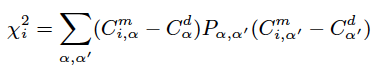
where Cα (α = 1–7) represents the projection coefficients. The superscript “m” and “d” refer to model and data. i represents the i-th model. Pα,α′ is the inverse of the covariance matrix of Cα. The covariance matrix of Cα is calculated in the projection process.
A weight wi = exp(-χi2/2) is defined to describe the similarity between the given galaxy and model i. A probability distribution function (PDF) is then built for each parameter P, by looping over all the model galaxies in the library and by summing the weights wi at the value of P for each model. The final PDF is normalized, and the parameter values at the 2.5, 16, 50 (median), 84 and 97.5 percentiles of the cumulative PDF are calculated. The median is adopted as the nominal estimation of P and the 16 – 84 percentile range of the PDF as its ±1σ confidence interval. The WMAP 7 flat ΛCDM cosmology with H0 = 70, Ωm = 0.274, and ΩΛ = 0.726. (White et al. 2011) is applied universally to each of the Portsmouth-Wisconsin-Granada computations by the BOSS Pipeline.
DATA
Data Release 13 is identical to Data Release 12 and was processed under GALAXY_VERSION v1_1.
Output is browsable via the Catalog Archive Server (CAS) database by selecting:
- Table stellarMassPCAWiscBC03
- Table stellarMassPCAWiscM11
FITS output files are available from BOSS_GALAXY_REDUX/GALAXY_VERSION, available at the SAS URL: https://data.sdss.org/sas/dr12/boss/spectro/redux/galaxy/v1_1.
You may download data based on the Wisconsin PCA datamodel from:
BC03:
- wisconsin_pca_bc03-DR12-boss.fits.gz [BOSS DR12],
- wisconsin_pca_bc03-26.fits.gz [SDSS DR8].
M11:
- wisconsin_pca_m11-DR12-boss.fits.gz [BOSS DR12],
- wisconsin_pca_m11-26.fits.gz [SDSS DR8].
REFERENCES
Brinchmann, J.; Charlot, S.; White, S. D. M.; Tremonti, C.; Kauffmann, G.; Heckman, T.; Brinkmann, J., 2004, MNRAS, 531, 1151 doi:10.1111/j.1365-2966.2004.07881.x
Bruzual, G.; Charlot, S., 2003, MNRAS, 344, 1000 doi:10.1046/j.1365-8711.2003.06897.x
Chen, Y.M.; Kauffmann, G.; Tremonti, C. A.; White, S.; Heckman, T. M.; Kovac, K.; Bundy, K.; Chisholm, J.; Maraston, C.; Schneider, D. P.; Bolton, A. S.; Weaver, B. A.; Brinkmann, J., 2012, APJ, 421, 314 doi:10.1111/j.1365-2966.2011.20306.x
Charlot, S.; & Fall, S. M., 2000, APJ, 539, 718 doi:10.1086/309250
Maraston, M.; & Strömbäck, G. , 2011, MNRAS, 418, 2785 doi:10.1111/j.1365-2966.2011.19738.x White, M.; Blanton, M.; Bolton, A.; Schlegel, D.; Tinker, J.; Berlind, A.; da Costa, L.; Kazin, E.; Lin, Y. T.; Maia, M.; McBride, C. K.; Padmanabhan, N.; Parejko, J.; Percival, W.; Prada, F.; Ramos, B.; Sheldon, E.; de Simoni, F.; Skibba, R.; Thomas, D.; Wake, D.; Zehavi, I.; Zheng, Z.; Nichol, R.; Schneider, D. P.; Strauss, M. A.; Weaver, B. A.; Weinberg, D. H. & White, M.; & 2011, APJ, 728, 126, doi:10.1088/0004-637X/728/2/126