
Examples
This page provides a series of potential science applications and then how to do those actions using tools and data products in the CAS (SQL), SAW (Web Application), and SAS (File Server, both IDL and Python). Some Python Tools are also provided in a Github Repository.
Science Applications
For each of the following science applications, we try to explain how one would go about investigating using the CAS (SQL), SAW (Web Application), and SAS (File Server, both IDL and Python). Where applicable, a "*" marks the preferred method for a given science application.
Users unfamiliar with the CAS (SQL) or SAW (Web Application) should consult the CAS tutorial and SAW tutorial sections on this page. For most of these science applications, "Using the SAS" means loading the entire allStar summary file into memory via IDL or Python, and manipulating data to suit the application. Python Tools are also provided in a APOGEE2 Tutorials Github Repository (though this work is in progress).
Spectral data is stored in FITS image files. There are standard packages in IDL and Python for using these files; useful information regarding using these files can be found here. All of our data models and, in consequence, the examples below assume a familiarity with these file formats.
Get Stellar Parameters and Abundances for the Main Red Star Sample
ASPCAP parameters, element abundances, and uncertainties for all stars in the main red star sample with reliable abundances.
- Following the advice on Using Stellar Parameters and Using Stellar Abundances , quantities that are not trustworthy will have a series of bits set in
APOGEE_ASPCAPFLAGorAPOGEE_STARFLAG. - Following the advice on Using Targets/Samples, the
APOGEE_EXTRATARGwill have no bits set if the star is in the main red star sample.
How to Select this Sample:
| Using the CAS (SQL) | Using the SAW (Web Application) | Using the SAS (File Server, IDL and Python) |
Get element abundances for stars flagged as known cluster members
Here, we provide an example of selecting objects chosen to be calibrator stars in clusters with known metallicities, which are identified with the APOGEE_CALIB_CLUSTER in either APOGEE_TARGET1 or APOGEE2_TARGET1 bit 9.
How to Select this Sample:
| Using the CAS (SQL) | Using the SAW (Web Application) | Using the SAS (File Server, IDL and Python) |
Building the H-R Diagram
ASPCAPFLAG options. Further constraints to the main red star sample or to exclude ancillary targets, for example, can be achieved by merging code from other examples.
How to Select this Sample:
| Using the CAS (SQL) | Using the SAW* (Web Application*) | Using the SAS (File Server, IDL and Python) |
Making an Abundance Plot
ASPCAPFLAG and also by removing errant values with a set of cuts. Second, it is advisable to sub-select regions of the galaxy. As in the H-R diagram example, further refinement of this sample can come from merging different examples on this page.
How to Select this Sample:
| Using the CAS (SQL) | Using the SAW (Web Application) | Using the SAS* (File Server*, IDL and Python) |
Investigating a Spectral Feature
To demonstrate using the spectra, we will look at an Ap star reported in Chojnowski et al. (2019). More specifically, we will use the star 2MASS J06010117+3214538 that is visualized in Figure 1 of Chojnowski et al. (2019).
The easiest way to visualize a spectrum is to use the SAW tools because it requires no detailed knowledge of the spectral data model (described in detail here). The SAW provides a means to overlay the spectral fitting windows used for ASPCAP, which is more than sufficient to ask if a spectral feature is problematic -- e.g., contaminated by a skyline or redshifted into a chip gap. Moreover, the SAW provides tools to investigate not only the combined spectra but also the visit spectra and the best-fit synthetic spectrum. Equivalent analyses in the SAS require the accumulation of several types of files in different locations as well as familiarity with each of their data models.
The SAW, however, does not provide analysis tools for line fitting or comparison outside of our standard analyses. For these tasks, the user can use the SAW to gather the data needed and then follow the SAS examples to perform additional investigation.
The SAW provides easy data download options for different spectral products that could be in several places within the SAS and may be more straight forward for acquiring spectral data.
No spectral access tools are provided in the CAS.
How to Perform this Investigation:
| Using the CAS (SQL) | Using the SAW* (Web Application*) | Using the SAS (File Server, IDL and Python) |
CAS Tutorials
Useful CAS Functions for APOGEE data
The CAS has several predefined table-based functions that can be used to return sub-sets of values from aspcapStar table, rather than having specifying each tag separately in a SELECT statement. These functions require a CROSS APPLY statement, but examples will be provided below.
| Function | Description |
|---|---|
dbo.fAspcapParamsAll |
returns all stellar parameters, uncertainties, and flags for the stellar parameter results |
dbo.fAspcapElemsAll |
returns all elemental abundances, their uncertainties, and their flags for the elemental abundance results |
| Sub-Function | Description |
dbo.fAspcapParams |
returns all stellar parameters |
dbo.fAspcapParamErrs |
returns uncertainties for all stellar parameters |
dbo.fAspcapParamFlags |
returns flags on the stellar parameters |
dbo.fAspcapElems |
returns abundances of all calibrated species |
dbo.fAspcapElemErrs |
returns uncertainties for all stellar elemental abundances |
dbo.fAspcapElemFlags |
returns flags on the elemental abundances |
Get Stellar Parameters and Abundances for the Main Red Star Sample
Limiting to the first 100 results (remove TOP 100 for full results), the CAS query is:
SELECT TOP 100 s.apogee_id, s.ra, s.dec, s.glon, s.glat, s.vhelio_avg, s.vscatter,
params.*, paramerrs.*, elems.*, elemerrs.*,
dbo.fApogeeAspcapFlagN(a.aspcapflag),
dbo.fApogeeStarFlagN(s.starflag)
FROM apogeeStar s
JOIN aspcapStar a on a.apstar_id = s.apstar_id
CROSS APPLY dbo.fAspcapParams(a.aspcap_id) params
CROSS APPLY dbo.fAspcapParamErrs(a.aspcap_id) paramerrs
CROSS APPLY dbo.fAspcapElems(a.aspcap_id) elems
CROSS APPLY dbo.fAspcapElemErrs(a.aspcap_id) elemerrs
WHERE (a.aspcapflag & dbo.fApogeeAspcapFlag('STAR_BAD')) = 0 and s.extratarg = 0
Get element abundances for stars flagged as known cluster members
Limiting to the first 100 results (remove TOP 100 for full results), the CAS query is:
SELECT TOP 100 s.apogee_id, s.ra, s.dec, s.glon, s.glat, s.vhelio_avg,
s.vscatter, a.teff, a.teff_err, a.logg, a.logg_err, a.m_h, a.m_h_err,
a.alpha_m, a.alpha_m_err, dbo.fApogeeAspcapFlagN(a.aspcapflag),
dbo.fApogeeStarFlagN(s.starflag)
FROM apogeeStar s
JOIN aspcapStar a on a.apstar_id = s.apstar_id
WHERE (a.aspcapflag & dbo.fApogeeAspcapFlag('STAR_BAD')) = 0 and s.commiss = 0
and (s.apogee_target2 & (dbo.fApogeeTarget2('APOGEE_CALIB_CLUSTER')) != 0)
Building the HR Diagram
Relaxing the target-selection criteria in the Main Red Star Sample example above will produce the catalog required in terms of stellar parameter quality.
Making an Abundance Plot
Relaxing the target-selection criteria in the Main Red Star Sample example above will produce the catalog required in terms of abundance quality.
Investigating a Spectral Feature
SAW Tutorials
Get Stellar Parameters and Abundances for the Main Red Star Sample
APOGEE2_TARGET1 bit 14 to ON. To select stars with no bits set in either APOGEE2_STARFLAG and APOGEE2_ASPCAPFLAG, select each bitmask and toggle STARFLAG = 0 and ASPCAPFLAG = 0. The result of this search is available here. An html table displayed on the page contains the results as well as means of obtaining the data or spectra.
Get element abundances for stars flagged as known cluster members
APOGEE_TARGET1 bit 9 (see here) and one for APOGEE2_TARGET1 bit 9 (see here). At this point, several download options are given for the data the user requires.
Building the HR Diagram
ASPCAPFLAG bits being set. Simply, navigate to the ASPCAPFLAG bit menu and select the "ASPCAPFLAG = 0" option for no bits set (lower right).
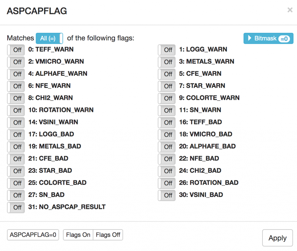
ASPCAPFLAG bit mask toggle display. In the bottom right, the "ASPCAPFLAG = 0" button will search for all stars with no bits set in this mask. Stated differently, these are all non-problematic spectra based on their ASPCAP fits.
The result of this search is here. Note: this search returns a large volume of visits and will take several minutes to complete; we, thus, advise users to follow the URL to find the results of the search.
On the display pane the "Table (csv)" button will start a download of a comma separated values formatted file with key information about the stars returned in the search. The top 10 lines of the file are provided below for inspection. This file includes basic location data, processing tags, and the stellar parameters array.
#apogee_id,location_id,field,apred_vers,apstar_version,aspcap_version,results_version,field,reduction_id,ra,dec,teff,teff_err,logg,logg_err,m_h,m_h_err,param_c_m,param_n_m,alpha_m,alpha_m_err,vmicro,aspcap_exists
'2M00000002+7417074','5046','120+12','r12','stars','l33','r12-l33','120+12','none','00:00:00.02','+74:17:07.47',3723.23,61.8,0.75,0.05,-0.15,0.01,-0.0,0.25,0.03,0.01,1.77,True
'2M00000019-1924498','5071','060-75','r12','stars','l33','r12-l33','060-75','none','00:00:00.20','-19:24:49.86',5508.86,110.27,4.31,0.09,-0.28,0.01,0.04,-0.16,0.08,0.01,0.8,True
'2M00000032+5737103','4264','N7789','r12','stars','l33','r12-l33','N7789','none','00:00:00.32','+57:37:10.31',6285.92,141.67,3.84,0.08,-0.18,0.03,0.09,0.0,0.07,0.02,1.99,True
This example can be combined with other bits, like targeting bits or STARFLAG bits to down-select the sample.
Building an Abundance Plot
The example above for "Building the HR Diagram" constructs a CSV file that has some of the required data for this exercise. We note that the $[Fe/H]$ and $[Mg/Fe]$ arrays are not provided by this interface. However, the $[\alpha/M]$ and $[M/H]$ parameters could be used instead to explore the data.
Investigating a Spectral Feature
Go to the Basic Search on the SAW. In the APOGEE ID field type '2M06010117+3214538' and click search.
The search should return 14 visits and 1 star for this search, which will be reported in the upper right of the search box when the search is complete. The result of this search can be found here.
The box below the search provides a number of visualization options:
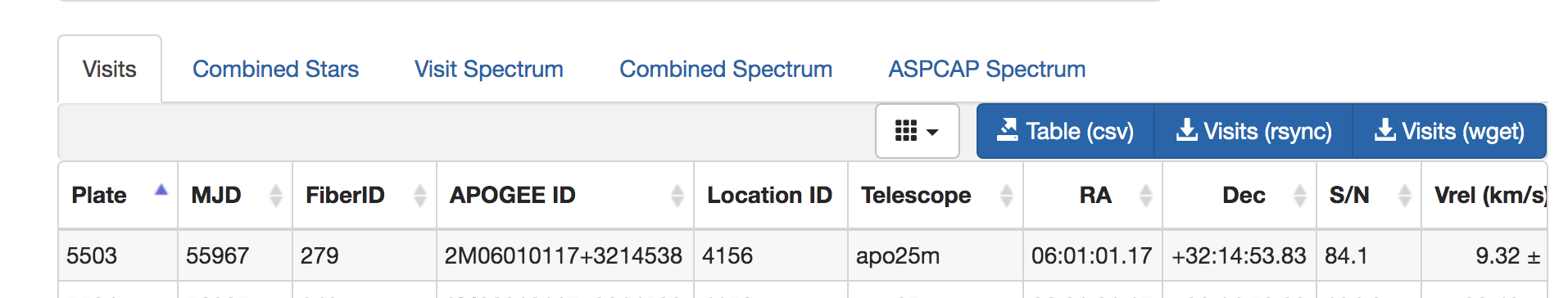
The Visits and Combined Stars tabs are provide the catalog-data derived from the spectral data. Catalogs can be downloaded as CSV files with the link Table (csv). The buttons for Visits (rsnyc) and Visits (wget) provide options for downloading the apStar/asStar spectra (the command and a download script with the SAS URLs for each star in the sample).
The tabs Visit Spectrum, Combined Spectrum, and ASPCAP Spectrum each provide interactive graphical interfaces for spectral visualization.
In the right-hand Search Options pane, the toggle for "Combined" versus "ASPCAP" will change the displace from the Combined spectrum (apStar/asStar) to the ASPCAP level analysis (aspcapStar). Parallel download options are provided for those data. The user can change that toggle and click Update to go between the two displays for the same underlying sample.
The Combined Spectrum tab displays summative properties for the star, including key bitmask parameters in the upper panel. The lower panel shows the combined spectrum with many plotting options that will overlay the corresponding sky spectrum and telluric spectrum, as well as overlaying spectral lines used in the ASPCAP analysis (the user can toggle on and off the lines of choice). An example visualization is given below. The light blue help box in the lower right provides instructions for interacting with the spectrum.
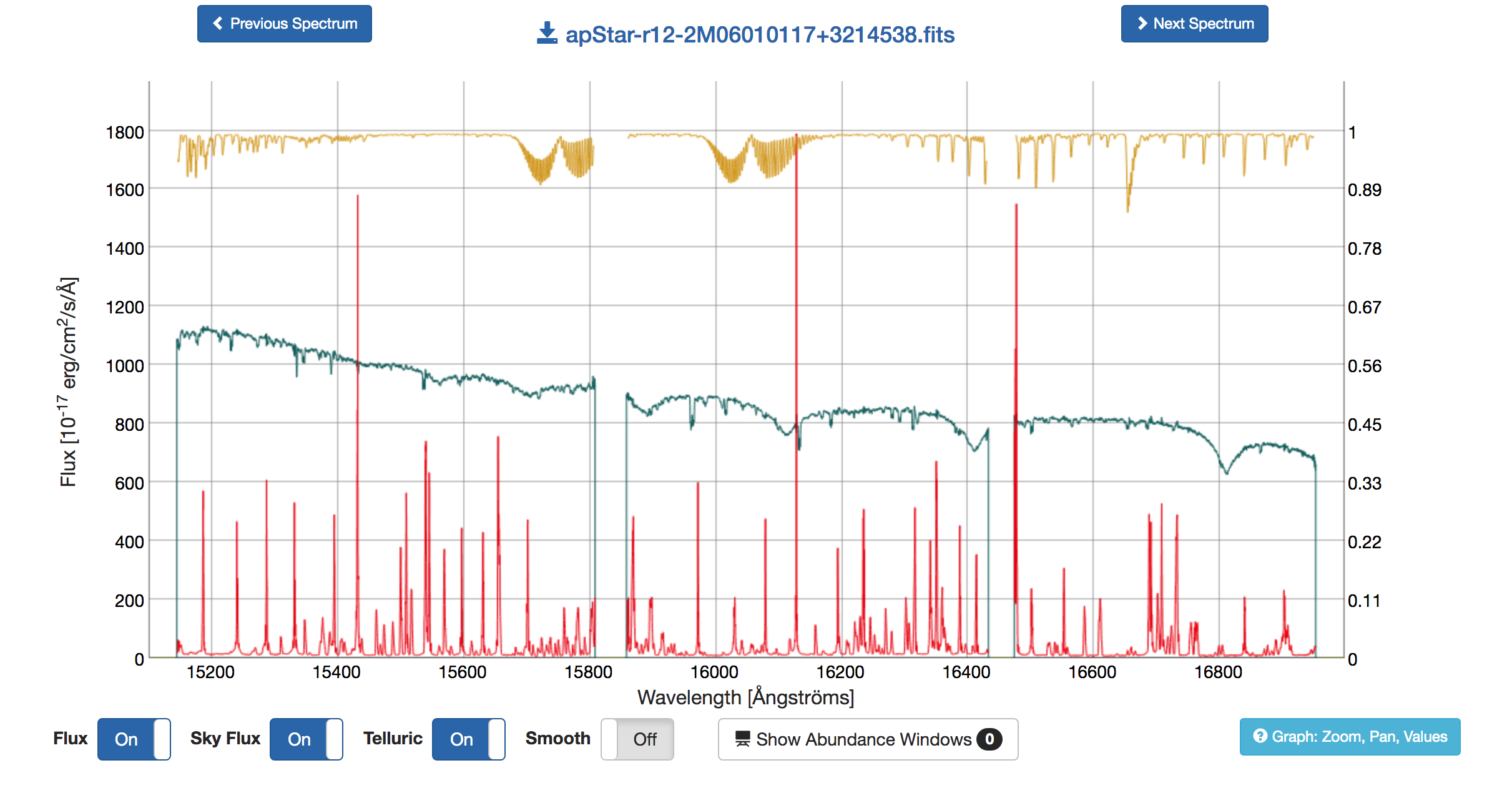
Similar interfaces are provided for the Visit Spectrum and ASPCAP Synthetic Spectrum. Of note for this star is the comparison between the stellar spectrum and the best fit ASPCAP spectrum, which is visible in the "ASPCAP Spectrum" tab. Here the unique features of this star are apparent.
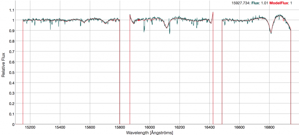
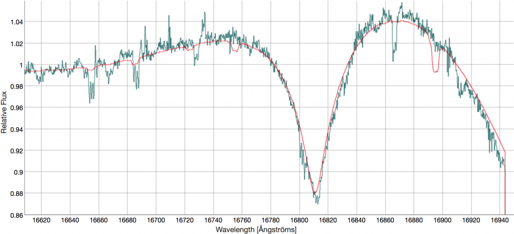
Comparing the panels above to Figure 1 of Chojnowski et al. (2019), the user can easily see how powerful the SAW tools are for spectral inspection and visualization.
SAS Tutorials
Some of the coding examples assume the user has SDSS Software. Lastly, while we do not provide examples on this page, the TOPCAT software is particularly good for working efficiently with the summary catalogs.
Get Stellar Parameters and Abundances for the Main Red Star Sample
allStar summary file loaded into IDL or Python as star and obtaining a sub-selection of stars in the gd array:
IDL
badbits = sdss_flagval('APOGEE_ASPCAPFLAG', 'STAR_BAD')
gd = where((star.aspcapflag and badbits) eq 0 and star.extratarg eq 0, ngd)
Python
import numpy
from astropy.io import fits (or import pyfits as fits)
star_hdus = fits.open('allStar-dr17-synspec.fits')
star = star_hdus[1].data
star_hdus.close()
badbits = 2**23
gd = (numpy.bitwise_and(star['aspcapflag'], badbits) == 0) & (star['extratarg']==0)
ind = numpy.where(gd)[0]
Get element abundances for stars flagged as known cluster members
allStar summary file loaded into IDL or Python as star and obtaining a sub-selection of stars in the gd array:
IDL
star = mrdfits('allStar-dr17-synspec.fits', 1)
badbits = sdss_flagval('APOGEE_ASPCAPFLAG', 'STAR_BAD')
clusterbits = sdss_flagval('APOGEE_TARGET2', 'APOGEE_CALIB_CLUSTER')
gd = where((star.aspcapflag and badbits) eq 0 and star.commiss eq 0 and $
    (star.apogee_target2 and clusterbits) ne 0, ngd)
Python
import numpy
from astropy.io import fits (or import pyfits as fits)
star_hdus = fits.open('allStar-dr17-synspec.fits')
star = star_hdus[1].data
star_hdus.close()
badbits = 2**23
clusterbits= 2**10
gd = (numpy.bitwise_and(star['aspcapflag'], badbits) == 0) &\
     (numpy.bitwise_and(star['apogee_target2'], clusterbits) != 0) &\
     (star['commiss'] == 0)
ind = numpy.where(gd)[0]
Making an HR Diagram
Using allStar summary file loaded into IDL or Python as star and obtaining a sub-selection of stars in the gd array:
IDL
Getting the Sample
 ; first, select for stars without flags
badbits = sdss_flagval('APOGEE_ASPCAPFLAG', 'STAR_BAD')
gd = where((star.aspcapflag and badbits) eq 0 and star.extratarg eq 0, ngd)
star = star[gd]
; second, clean up any errant values
gd_val = where(star.TEFF gt 0 and star.LOGG gt -10 and star.FE_H gt -6)
star = star[gd_val]
Plotting
This makes a simple plot using the sample defined above. More complex plotting tutorials can be found here.
plot,star.TEFF,star.logg,psym=3,xr=[6500,3000],yr=[6.5,-0.5],xstyle=1,ystyle=1,xtit='Teff [K]',ytit='log(g) dex'
Python
Getting the Sample
 #!/usr/bin/env python
# coding: utf-8

import fitsio
from matplotlib import pyplot as plt
import numpy as np
data = fitsio.read("allStar-dr17-synspec.fits")

starbad = 2**23 #bit flag for bad stars
gd = np.bitwise_and(data["ASPCAPFLAG"], starbad) == 0
teff_logg_check = np.logical_and(data["TEFF"] > 0, data["LOGG"] > -10) # this checks for -9999 values
teff_logg_feh_check = np.logical_and(data["FE_H"]> -6, teff_logg_check)

indices = np.where(np.logical_and(gd, teff_logg_feh_check))
good = data[indices] # this only the good data now
Teff_vals = good["TEFF"]
logg_vals = good["LOGG"]
FeH_vals = good["FE_H"]
Plotting
#plotting the HR Diagram
fig = plt.figure(figsize=(12,12))
ax = fig.add_subplot(111)

image = ax.scatter(Teff_vals,logg_vals, c=FeH_vals ,edgecolor='k',cmap="plasma",alpha=0.5)
bar = fig.colorbar(image,orientation="vertical",pad=0.01)
bar.set_label('$[Fe/H]
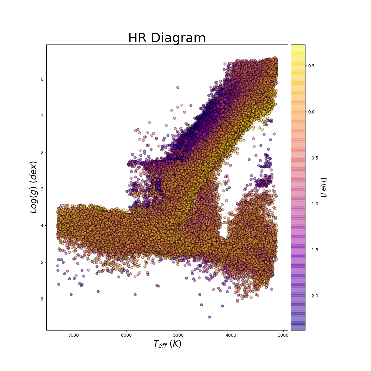
Plot by John Donor & Taylor Spoo.
Making an Abundance Plot
allStar summary file loaded into IDL or Python as star and obtaining a sub-selection of stars in the gd array:
IDL
Getting the Sample
 ; first, select for stars without flags
badbits = sdss_flagval('APOGEE_ASPCAPFLAG', 'STAR_BAD')
gd = where((star.aspcapflag and badbits) eq 0 and star.extratarg eq 0, ngd)
star = star[gd]
; second, clean up any errant values
gd_val = where(star.MG_FE gt -6 and star.FE_H gt -6)
star = star[gd_val]
Now define samples for inner and outer galaxy:
inner_gal = where((star.glon ge 350. or star.glon le 10) and abs(star.glat) lt 5)
outer_gal = where((star.glon gt 90. or star.glon le 270) and abs(star.glat) gt 10)
Plotting
This makes a simple plot using the sample defined above. More complex plotting tutorials can be found here.
!p.multi=[0,1,2,0]

plot,star[inner_gal].FE_H,star[inner_gal].MG_FE,psym=3,xr=[-2.5,0.75],yr=[-1.,1.25],xstyle=1,ystyle=1,xtit='[Fe/H]',ytit='[Mg/Fe]'

plot,star[outer_gal].FE_H,star[outer_gal].MG_FE,psym=3,xr=[-2.5,0.75],yr=[-1.,1.25],xstyle=1,ystyle=1,xtit='[Fe/H]',ytit='[Mg/Fe]'
Python
Getting the Sample
 #!/usr/bin/env python
# coding: utf-8
import fitsio
from matplotlib import pyplot as plt
import numpy as np
data = fitsio.read("allStar-dr17-synspec.fits")

starbad = 2**23
gd = np.bitwise_and(data["ASPCAPFLAG"], starbad) == 0
i_cut = np.logical_or(np.abs(data["GLON"])>=350, data["GLON"]<=10)
l_bsmall_check = np.logical_and(np.abs(data["GLAT"])<5, i_cut)

o_cut = np.logical_and(np.abs(data["GLON"])>90, data["GLON"]<270)
l_bbig_check = np.logical_and(np.abs(data["GLAT"])>10, o_cut)

abun_good = np.logical_and(data["FE_H"]>-6, data["MG_FE"]>-6)

l_bsmall_Feh_check = np.logical_and(l_bsmall_check, abun_good)
l_bbig_Feh_check = np.logical_and(l_bbig_check, abun_good)
ind_1 = np.where(np.logical_and(gd, l_bsmall_Feh_check))
ind_2 = np.where(np.logical_and(gd, l_bbig_Feh_check))

good1 = data[ind_1]
good2 = data[ind_2]

alpha1 = good1["MG_FE"]
FeH1= good1["FE_H"]

alpha2= good2["MG_FE"]
FeH2 = good2["FE_H"]
Plotting
 #plotting
fig = plt.figure(figsize=(16,8))

ax1 = fig.add_subplot(121)
image1 = ax1.scatter(FeH1, alpha1, c="m" ,edgecolor='k',alpha=0.3)
ax1.set_xlabel("[Fe/H]", size=20)
ax1.set_ylabel("[Mg/H]", size=20)
ax1.set_title("inner galaxy", size=30)

ax2 = fig.add_subplot(122)
image2 = ax2.scatter(FeH2, alpha2, c="c", edgecolor='k', alpha=0.3)
ax2.set_xlabel("[Fe/H]", size=20)
ax2.set_ylabel("[Mg/H]", size=20)
ax2.set_title("outter galaxy", size=30)
plt.savefig("alpha_fe.png")
![Plot of the [Mg/Fe] against [Fe/H] for the DR17 sample using the example python code.
<em>Plot by John Donor & Taylor Spoo.</em>](/wp-content/uploads/2019/11/alpha_fe.png)
Plot by John Donor & Taylor Spoo.
Investigating a Spectral Feature
Obtain Spectra
There are two ways to obtain the spectrum. First, the spectrum can be downloaded directly from the SAW. A single spectrum can be downloaded from its spectrum display in the SAW (the file name, itself, is the download link). Alternately, bulk downloads can be accomplished using the catalog search tools and using the rsync or wget options in the upper left of the display.
Second, the spectrum can be downloaded from the SAS and the user needs to build the SAS URL as described on Data Access for Spectral Data.
The apStar (data model) file for this star can be found at the following URL:
https://data.sdss.org/sas/dr17/apogee/spectro/redux/dr17/stars/apo25m/180+04/apStar-dr17-2M06010117+3214538.fits
The URL can be built from the base URL for the apStar spectra:
/sas/dr17/apogee/spectro/redux/dr17/stars/
with the values for TELESCOPE, FIELD, and APOGEE_ID taken from a summary table or from the SAW display.
The user may want to also use other Spectral Data products, like the ASPCAP model file (aspcapStar). Information on Data Access can be used to understand the data formats and access those data.
Reading in Spectral Data
The following example uses an apStar file. If using a different data format (say, aspcapStar), then these examples will need to be modified.
In this example, the spectral data is held in the variable, f. For apStar/asStar filetypes, f is an image array. For apStar/asStar files, there are multiple spectra in f; first, the combined spectrum and then, each of the individual visit spectra. apStar/asStar files have data in flux units, whereas the aspcapStar file contain the normalized spectra used for ASPCAP analysis (the spectrum divided by a fit to the continuum).
IDL
f = mrdfits('apStar-dr17-2M06010117+3214538.fits’,1,hdr)
;HDU contains combined spectra, then each visit spectra as an array, use the 0th element of the image array (data) to get the combined spectrum.
f = reform(data[*,0])
nf = nelements(f)

crval1 = double(sxpar(hdr,'CRVAL1'))
cdelt1 = double(sxpar(hdr,'CDELT1'))
wave = dindgen(nf)

wave=crval+(cdelt*wave)
wave = 10**wave
restwave=wave-((vhelio/299792.458e0)*wave)

plot,w,f
Python
An example of reading in a apStar file and producing the rest-frame wavelength axis is given below. It assumes that the radial velocity VHELIO has already been obtained to shift the observed wavelength to the rest frame.
import numpy as np
from astropy.io import fits, ascii

### Read in file for magnetic star; get flux and rest frame wavelengths

spec='apStar-dr17-2M06010117+3214538.fits'
star='2M06010117+3214538'

f=fits.getdata(spec)
hdr=fits.getheader(spec)
nf=len(f)
crval=np.double(hdr['CRVAL1'])
cdelt=np.double(hdr['CDELT1'])
w=np.empty(nf)

for k in range(nf): w[k]=crval+(cdelt*k)
w=10.0**w

w=w-((vhelio/299792.458e0)*w)

plt.plot(w,f)
With the spectral data and wavelength array in hand, the user can produce figures by the means most comfortable for them. However, there are a few useful items that can help with spectral visualization.
Spectral Inspection
There are two ways to inspect part of a spectrum. Following the appropriate data model for the spectral data, the actual subtracted sky spectrum is available for each visit. Alternately, users may wish to plot against this list of known airglow lines (from the APOGEE software Github Repository). To further evaluate spectra, the spectral windows used in ASPCAP are available for each element can also be found in the windows section of the APOGEE Software Github Repository.