Using Radial Velocities
This page has important information about using the DR16 APOGEE combined and individual visit radial velocities (RVs) and provides several examples to illustrate their uses. An understanding of how the quality of the supplied measurements are flagged using bitmasks is important to properly and effectively utilize these datasets.
Visit-level Radial Velocities
For each visit to an object, APOGEE reports the relative RV as VREL and the associated uncertainty is stored in VRELERR. The barycentric correction is given by BC, and applied to the relative RV to yield the visit barycenter-corrected velocity, VHELIO. Because the barycentric correction can be calculated very precisely (at the m/s level), the uncertainty for VHELIO is VRELERR. An integer value of the Modified Julian Date on which that star was observed is given by MJD (see Nidever et al. 2015). If one is interested in utilizing the visit RVs to search for variations in RV over time, one should look for variations in VHELIO as a function of the Julian Date JD. The Julian Date in summary files is the JD-MID from the apVisit file, which refers to the middle of an exposure sequence (a "visit") determined from exposure-time weighted mean of the mid-exposure times and the exposure times are nearly always the same. For RV-variations on timescales shorter than a typical "visit" (normally, ~80 min including overheads), this may be insufficient time resolution. Please see APOGEE Visit Reduction for additional details about the derivation of visit-level RVs.
At the visit-level, the STARFLAGS bitmask provides detailed quality information about the individual visit spectra. Results from any visit that has the LOW_SNR flag, which is set automatically for all spectra with signal-to-noise (SNR) less than 5, should not be included in any analysis. We note that, ideally, a lower limit on the SNR of ~10 will produce the best results. Additionally, visits with either the BAD_PIXELS and VERY_BRIGHT_NEIGHBOR flags should not be used. These three flags are the most obvious indicators that the visit RV may not be trustworthy, but for the highest quality visit velocities, one should also exclude visits with PERSIST_HIGH, PERSIST_JUMP_POS, and PERSIST_JUMP_NEG. Other STARFLAGS or additional cuts based on VRELERR (e.g., all visit velocities must have uncertainties less than 10 km/s) may be utilized to further remove RVS determined from low-quality visit spectra.
Please see Nidever et al. 2015 for a detailed discussion of the pipeline. Both Troup et al. 2016 and Price-Whelan et al. 2018 provide more detailed examples of using the visit-level APOGEE RVs for scientific analyses.
Average Radial Velocities
APOGEE also reports the SNR weighted average velocity as determined from the combined spectra. This is recorded as VHELIO_AVG and the scatter around this average is stored in VSCATTER. The number of visit spectra included in the combined spectra is given by NVISITS. Please note that the number of visits given for the combined spectra (e.g., in allStar file) does not always match the total number of visits obtained (e.g., the number of unique entries in the allVisit file); this is a known aspect of the reduction pipeline. An object that was observed on two different plates will be passed through the visit-combination pipeline as two distinct objects and, thus, will be presented as separate entries in catalogs containing combined data; the object will have the same APOGEE_ID, but with different field tags (the sum of field and APOGEE_ID define a unique object for which visit spectra are combined). The number of visits recorded for a combined spectrum will always correspond to the number of visits contributing to that combination. The sum of the NVISITS for each entry of that object will be equal to the total number of visits across all fields (e.g., the number of unique observations present at the visit level).
The SNR weighted uncertainty is stored in VERR and the median visit RV uncertainty is stored in VERR_MED. These uncertainties are known to be underestimated; in some cases, e.g., a combined spectrum with high-SNR obtained over many visits, VSCATTER may represent a better estimate of the overall measurement precision. If VSCATTER is very large (i.e., much larger than VERR_MED) and measured from multiple (more than 3) high-SNR visit spectra, this may be an indicator that the star is in a stellar binary. For stars with only a single visit, VSCATTER is set to zero.
Both Visit Combination and Radial Velocities pages provide detailed outlines of the visit combination and average RV derivation process.
Example: Eclipsing Binary KIC 2161623
KIC 2161623 (APOGEE_ID 2M19265867+3735276) is a known eclipsing binary discovered by Kepler (see Conroy et al. 2014 for details) that has a period of 2.2835 days (Kirk et al. 2016). This star has been observed by the APOGEE survey with a total of 20 visits (each with SNR > 10), resulting in a combined spectrum with high signal-to-noise (SNR ~ 160).
In this example, we assume a user wants to (1) confirm that the star is in a binary system, and (2) derive its orbital period using only the data provided by APOGEE.
VSCATTER to the measurement error. For KIC 2161623, the VSCATTER is ~100 km/s, which is much greater than the median visit RV error (< 1 km/s), so it can be inferred that the star is a binary.
In general, if VSCATTER > 1 km/s (and VSCATTER is more than ~5×VERR_MED), the star is likely a binary; however, if a star has only a few visits or many very low-SNR (< 5) visits, VSCATTER may not be a reliable indicator of binarity. For this reason, a large value for VSCATTER is not a definitive marker for binarity; individual systems should be studied more closely for this determination.
Note also, in the allStar file, the SUSPECT_RV_COMBINATION STARFLAG is set for this star. This warning flag might be set when the pipeline has to use large RV offsets to create the combined spectra. Depending on the user’s goals, this flag may be essential, or it may be ignored. In this case, the flag can be ignored, since a large RV variation should be expected for such a short-period, stellar binary.
From the allVisit file, the STARFLAGS should be used to filter out low-SNR or poor-quality visits. For KIC 2161623, only two of the 20 visits have any flags set; those two visits both have the PERSIST_LOW flag set, which is a low-level warning flag that can be ignored for this purpose. The user should consider whether this flag will be ignored in all or some cases. Additionally, the user should check that the uncertainties are suitable for this analysis. In this case, the VRELERR given for each visit is < 2 km/s; again, the measurement errors are much less than the scatter, so all 20 visits can be included.
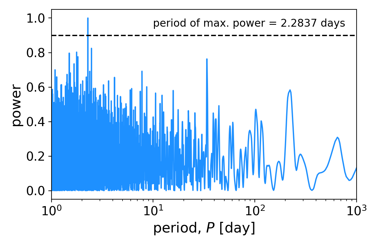
Using the visit RVs (VHELIO) and the associated errors, a Lomb-Scargle periodogram (Press & Rybicki 1989) can be used to detect periodic signals in the observations. The period of maximum power in the periodogram for this set of observations falls at 2.2837 days, so the APOGEE RVs confirm the period derived from the Kepler transits of the system.
Users interested in fitting other orbital parameters (e.g., semi-amplitude, eccentricity, etc.), might use one of the various available RV variation fitters. RV variation fitters include, but are not limited to: RadVel (Fulton et al. 2018), Systemic Console (Meschiari et al. 2009), and The Joker (Price-Whelan et al. 2017).
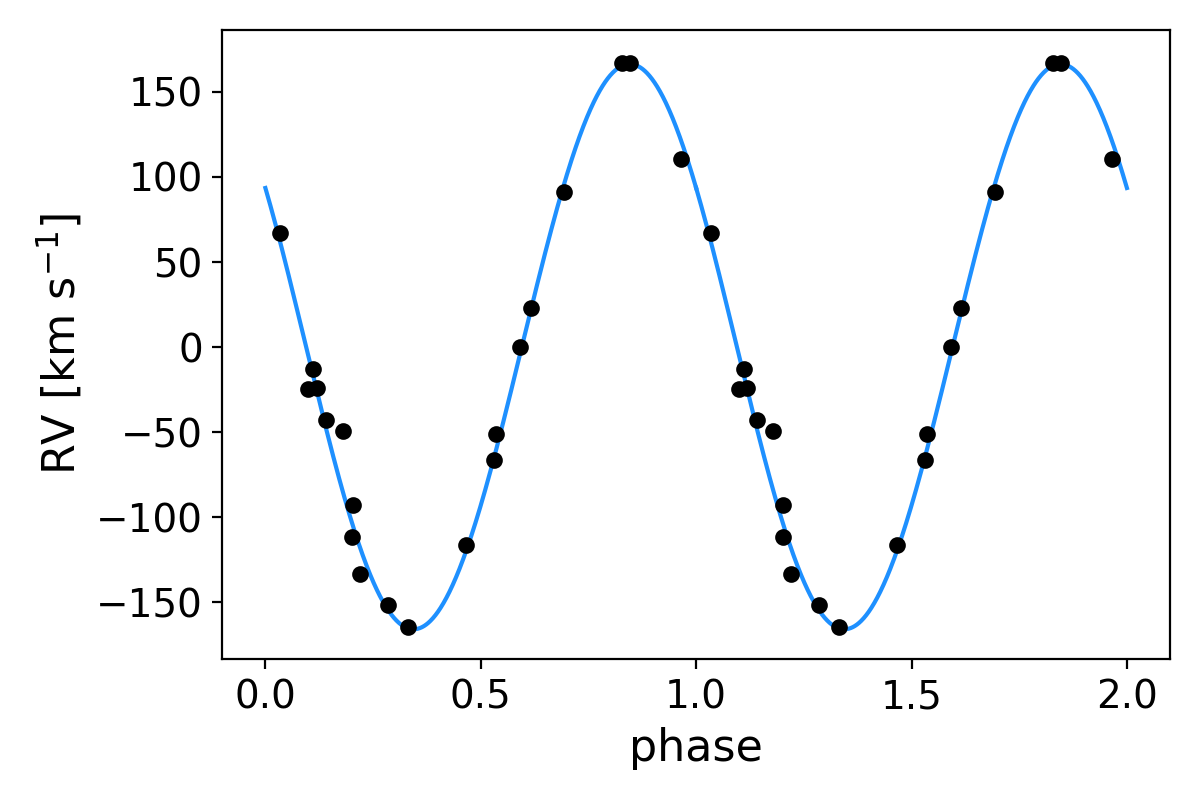
With 20 visits, all of these algorithms should converge on a single orbital solution for KIC 2161623. The user will find a low-eccentricity orbit (e < 0.01), with a period of 2.2837 days and a semi-amplitude of 166 km/s. The derived systemic velocity for the system is v0 = -46.2 km/s, whereas the SNR weighted average velocity is VHELIO_AVG = -66.6 km/s with VERR_MED = 0.7 km/s. The systemic velocity is not within the RV uncertainty but is well within the scatter of the data. The phase-folded orbit is shown below.
Both Troup et al. 2016 and Price-Whelan et al. 2018 provide more detailed examples of using the visit-level APOGEE RVs for scientific analyses.