A tutorial based on the LVM data preview for the Helix Nebula can be found in the “lvm_dr19_helix_nebula_tutorial” directory of this GitHub repository It requires the lvmSFrame-00004297.fits file as input, which can be obtained here. As always, do also consult the LVM caveats before you start working with the data.
The tutorial focuses on this reduced and calibrated LVM data. It teaches one how to:
- Access the fits file and display the list of Header Data Units
- From the fits file, extract the slitmap table; and from this table, extract the data for fibers without known problems and load it into a data frame
- Display a table with the slitmap
- Make a map of fibers without known issues with fiber-id labels
- Correct wavelength array for Doppler shift
- Obtain index of flux array corresponding to fiber of interest
- For a fiber of given ID, plot the reduced spectrum including the flux errors
- Zoom into spectral regions around Hα and Hβ in the observed and rest frames, note the presence of bad columns
- Note that some fibers capture bright stars
- Make maps of the emission within spectral windows around emission lines
- Make a composite RGB (red/green/blue) map that combines fluxes from three different spectral windows that capture emission lines
- Fit a single Gaussian to an emission line to obtain its flux
- Make an emission-line ratio map based on Gaussian fits to the lines
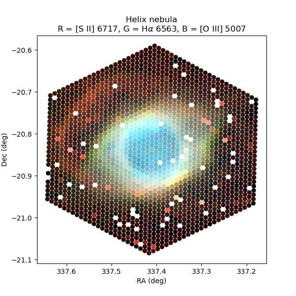
Composite red (R), green (G), blue (B) map of the Helix nebula constructed by using spectral windows that capture the three emission lines given in the title. Fibers with known issues have been removed. We include fibers that catch contaminating stars.