Summary
BOSSNet determines stellar parameters for BOSS spectra using a 1D residual convolutional network. For a complete description, please see Sizemore et al. (2024). The model was trained on both BOSS and LAMOST spectra, interpolated onto a common 3900 element wavelength grid ranging uniformly from 3800 to 8900 Å, approximating the typical resolution of the data within that range. The LAMOST data were used to ensure that sufficient labels were available across the HR diagram, as the MWM BOSS data currently has limited overlap with APOGEE and other datasets with well-determined stellar parameters.
Detailed Description
BOSSNet uses an extensive training set (Figures 1 & 2) resulting in a comprehensive coverage between 1700 < Teff < 100,000 K and 0 < log g< 10, to ensure BOSS Net can reliably measure parameters of most of the commonly observed objects within this parameter space.
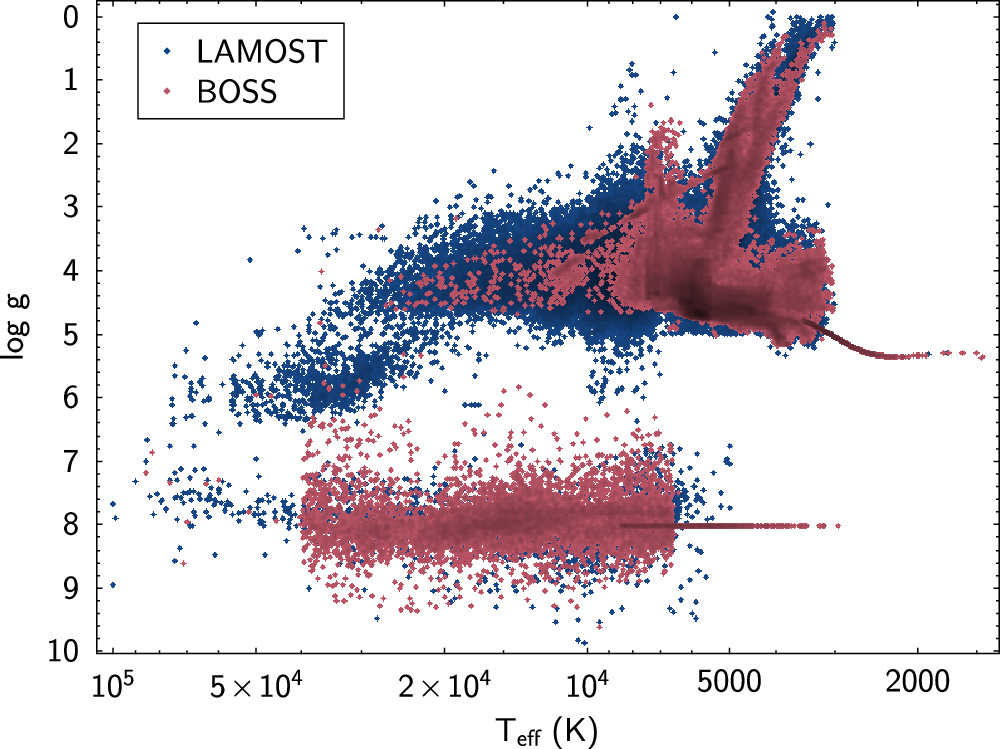
Figure 1: Sizemore et al. (2024) showing the BOSSNet training set.
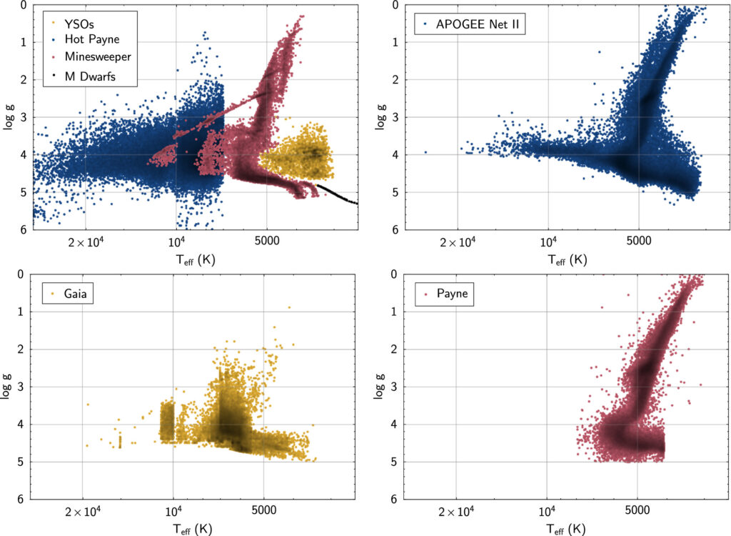
Figure 2: Sizemore et al. (2024) showing subsets of the BOSSNet training set.
BOSS Net is a 1D residual convolutional network consisting of a series of 1D convolutional Residual Network blocks and a final linear network for prediction.
The BOSS Net model takes a star’s spectrum as input. To regularize and avoid overfitting, data augmentation techniques are employed, such as randomly removing continuous segments of flux, dropping specific values in the flux, and adding noise to the flux by scaling a normal distribution sample by the error.
The model starts with a single convolutional block that includes a 1D convolutional layer, batch normalization, an Exponential Linear Unit (ELU) activation function, and a 1D max pooling layer (Figure 4). Batch normalization helps to improve the speed and stability of the training process by normalizing the inputs to each layer, reducing covariate shift, which is the change in input distribution of model layers as the model trains (Ioffe & Szegedy 2015). The ELU activation function enhances the performance and convergence speed of the model compared to other activation functions such as Rectified Linear Units (ReLU; Clevert et al. 2015). The max pooling layer helps reduce the number of parameters in the model, which can prevent overfitting and improve generalization to unseen data. Additionally, the model includes a positional encoding as a channel to the first convolutional layer of the first block, allowing for a more effective capturing of local patterns in the spectra at a given wavelength.
The output from the initial convolutional block flows into the first of many Residual Neural Network (ResNet) blocks. Each block consists of two 1D convolutional layers, each with batch normalization and an ELU activation function. The residual connection in this block allows the network to learn the residual mapping from the input to the output rather than the complete mapping, which can help with the vanishing gradient problem during training. ResNets were designed to allow for easier flow of information and gradients throughout the network, enabling the training of deeper models (He et al. 2016).
After the output of the residual blocks is obtained, it is passed through an adaptive average pooling layer. This layer serves to adjust the dimensions of the outputs to a fixed size, allowing for easier integration with the final linear network. The outputs of the adaptive pooling layer are then fed into several linear layers, each followed by the ReLU activation function. The final linear network provides the model prediction for the star’s Teff, , [Fe/H], and RV.
BOSS Net is evaluated with the mean squared error between the predicted and actual values. To encourage accurate modeling of the less populated regions of the parameter space, the loss of stars was adjusted, either by increasing or decreasing their weight in the loss calculation during training. The weight of specific regions is determined by the reciprocal of the Kernel Density Estimation (KDE) values computed from the training labels. This allows the model to prioritize the learning of less common samples, as indicated by their low-density regions in the KDE estimation, while reducing the impact of well-modeled samples, which are associated with high-density regions. As shown in Figure 5, the white dwarfs and the hot subdwarfs are weighted higher in the loss calculation, as they are in less dense regions of the parameter space. In addition, [Fe/H] of metal-poor stars is weighted higher in comparison to the metal-rich stars, and RVs of WDs or stars with RV > 200 km s−1 are weighed higher than for other sources, once again due to their rarity in the sample. The model was trained with a learning rate of 0.0001 using the Adamax optimizer (which is more robust to the presence of outliers; Kingma & Ba 2014), and a batch size of 512.
Data Products
In Data Release 19, BOSSNet is executed on all BOSS `mwmStar` (star- and telescope-combined spectra) and `mwmVisit` (individual visit) spectra.
There are two key data products produced by BOSSNet and Astra:
- `astraAllStarBossNet`: this file contains stellar parameters based on combined spectra in the `apStar` files
- `astraAllVisitBossNet`: this file contains stellar parameters based on visit spectra in the `apStar` files
Validation and Uncertainties
Figure 3 (Sizemore et al. 2024) shows the performance of BOSSNet
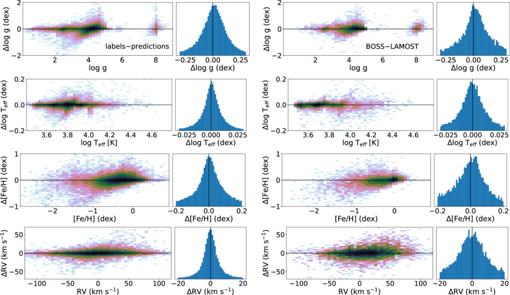
Please see the Discussion Section in Sizemore et al. (2024) for additional validation plots.
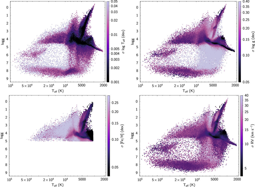
Sizemore et al. (2024) derived the uncertainties (Figure 4) in the predictions by generating 20 different realizations of the same spectrum by scattering the input fluxes by the reported uncertainties. All these realizations are separately passed through the model. The scatter in the resulting predictions is then evaluated and adopted as the uncertainties. These uncertainties are model dependent and are not representative of systematic errors that can be assessed through comparison to external data sets. However, the reported uncertainties do provide meaningful variance.
Flags
| Field Name | Bit | Flag Name | Flag Description |
result_flags | 0 | RUNTIME_EXCEPTION | Exception occurred at runtime |
result_flags | 1 | UNRELIABLE_TEFF | teff is outside the range of 1700 K and 100,000 K |
result_flags | 2 | UNRELIABLE_LOGG | logg is outside the range of -1 and 10 |
result_flags | 3 | UNRELIABLE_FE_H | teff < 3200 K or logg > 5 or fe_h is outside the range of -4 and 2 |
result_flags | 4 | SUSPICIOUS_FE_H | [Fe/H] below teff < 3900 K and with 3 < logg < 6 may be suspicious |
flag_warn | — | WARN | If UNRELIABLE_FE_H or SUSPICIOUS_FE_H are set. |
flag_bad | — | BAD | If any of these flags are set: UNRELIABLE_TEFF, UNRELIABLE_LOGG, UNRELIABLE_FE_H, RUNTIME_EXCEPTION. |