LVM Tutorials

This page describes the set of tutorials provided for the SDSS-V Local Volume Mapper (LVM) products released in DR20. The tutorials are distributed as Jupyter notebooks in the dedicated DR20 tutorials repository:

https://github.com/sdss/dr20_tutorials

The notebooks cover the two main families of LVM data products released in DR20: the reduced row-stacked spectra (lvmSFrame files, lvmSFrame-EXPNUM.fits) produced by the LVM Data Reduction Pipeline (DRP), and the higher-level analysis products (dap-rsp108-sn20-EXPNUM.dap.fits files) produced by the LVM Data Analysis Pipeline (DAP). They illustrate, in self-contained examples, how to read these files, how to combine them across exposures into mosaics, how to regenerate the spectral models from the DAP outputs, and how to apply the quality-control flags. Most examples use the Helix Nebula exposure (MJD = 60191, EXPNUM = 4297) as their primary dataset, but the workflows are broadly applicable to any DR20 LVM exposure.

As always, do consult the LVM caveats and the DR20 LVM quality-control information before working with the data.

Tutorial Index

• 1. DR20 Helix Nebula SFrame tutorial first contact with a reduced LVM exposure.
• 2. Interactive SFrame viewer interactive inspection of lvmSFrame files.
• 3. Helix Nebula DAP tutorial reading and exploring a single DAP file.
• 4. Mosaic DAP tutorial combining multiple DAP files into a mosaic.
• 5. DAP output-model generation reconstructing the spectral models from the DAP outputs.
• 6. DAP model-file reading and plotting
• 7. Quality-control bitmask tutorial reading and applying the LVM QC flags.

---

1. DR20 Helix Nebula SFrame tutorial

Notebook: lvm_dr20_helix_nebula_tutorial.ipynb
Dataset: SDSS-V LVM SFrame for the Helix Nebula (MJD = 60191, EXPNUM = 4297); DRP version version using DRP 1.2.0.

This is the entry-level tutorial for any user new to the LVM data products. It uses the reduced and calibrated lvmSFrame file of the Helix Nebula and walks through the full sequence required to extract a usable, science-ready spectrum from an LVM exposure. The tutorial originated as the only example provided with DR19 and has been refreshed for DR20 to use the updated DRP reduction.

The notebook teaches how to:

1. access the FITS file and display the list of Header Data Units;
2. extract the SLITMAP table, select the science fibers without known problems, and load them into a data frame;
3. display a table with the fiber map;
4. build a fiber map with fiber-id labels and a highlighted central fiber;
5. correct the wavelength array for the Doppler shift of the source;
6. obtain the index in the flux array corresponding to a fiber of interest;
7. plot the reduced spectrum of a selected fiber, including the flux errors;
8. zoom into spectral regions around Hα and Hβ in the observed and rest frames, and recognize the presence of bad columns;
9. identify fibers that capture bright contaminating stars;
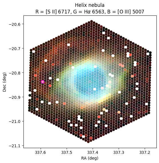
10. build maps of the emission integrated within narrow spectral windows around individual emission lines;
11. build a composite RGB map combining three emission-line spectral windows;
12. fit a single Gaussian to an emission line to obtain its flux;
13. build emission-line ratio maps, e.g., Hα/Hβ, from the Gaussian fits.

---

2. Interactive SFrame viewer

Notebook: lvm_dr20_SFrame_view.ipynb
Dataset: SDSS-V LVM SFrame for the Helix Nebula (DRPVER = 1.2.0, MJD = 60191, EXPNUM = 4297).

This notebook complements the basic SFrame tutorial above by providing an interactive widget-based viewer for the same kind of lvmSFrame products. It is built on top of matplotlib in widget mode and ipywidgets, and is designed to let users move quickly between the spatial and the spectral views of an LVM exposure.

The notebook teaches how to:

1. load an SFrame product using sdss_access/sdss-tree, with a local path fallback when needed;
2. read the position table of the science fibers and select the good-quality science fibers from the SLITMAP;
3. build an ERROR extension on the fly from the IVAR array and inspect the resulting HDU list;
4. reconstruct narrow-band slices directly from the row-stacked spectra to produce pseudo-images for individual emission lines (Hα, [O III], [N II]);
5. use the interactive viewer to explore fiber spectra and sky maps simultaneously, switch wavelength windows, and adjust flux scales and colormaps;
6. export selected subsets of fibers to a new FITS structure, preserving the standard SFrame extensions (FLUX, IVAR, MASK, WAVE, LSF, SKY, SKY_IVAR, SLITMAP) for further analysis.

The viewer combines two main panels a sky-map panel on the left and a spectral panel on the right. Left-clicking on the map adds fibers to the current selection and updates the average spectrum on the right; right-clicking removes fibers from the selection; holding the middle mouse button moves a “nearest fiber” cursor that lets you scan the field. On the spectral panel, selecting a wavelength range with the mouse buttons updates the map to show the average flux integrated over that range. Bottom panels control the spectral and flux ranges and allow saving snapshots.

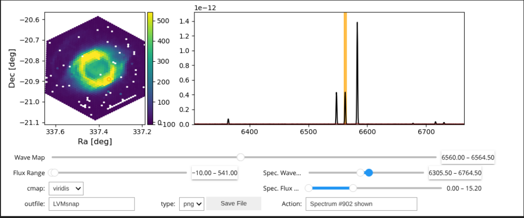
A complementary video tutorial walking through the use of this interactive viewer is available at:

---

3. Helix Nebula DAP reading tutorial

Notebook: lvm_dr20_helix_nebula_DAP_tutorial.ipynb
Dataset: SDSS-V LVM DAP file for the Helix Nebula (DRPVER = 1.2.0, DAPVER = 1.2.0.251218, MJD = 60191, EXPNUM = 4297).

This is the main tutorial for users who want to work with the LVM DAP data products. It documents the process of generating the figures shown in Sanchez et al. (2025) on the Helix Nebula using the per-exposure DAP file as the only input. The notebook is the recommended starting point to learn how to combine the parametric and non-parametric measurements, the stellar-population products, and the per-fiber position table that the DAP delivers.

The notebook teaches how to:

1. open and inspect a DR20 DAP product, both via sdss_access and from a local directory, and identify the content of every extension (PT, RSP, COEFFS, PM_ELINES, NP_ELINES_B/R/I, PM_KEL, ELINES_SIGMA_CHI, ELINES_CHI2_AVG, INFO);
2. build RGB emission-line maps that combine three different tracers into a single quick-look image, separately for the first parametric (pe), the second parametric (pek), and the non-parametric flux measurements;
3. build RGB maps of faint diagnostic and auroral lines ([N II] 5755, Hε, [O III] 4363, [S III] 9531), illustrating the depth and uniformity of the DAP analysis across the full LVM wavelength range;
4. construct the classical BPT/Veilleux Osterbrock diagnostic diagrams on a fiber-by-fiber basis (log [O III]/Hβ vs. log [N II]/Hα, log [S II]/Hα, log [O I]/Hα, and log [O II]/Hβ), with color coding consistent with the RGB maps;
5. build an integrated emission-line catalog from the per-fiber DAP products by summing fluxes across the field, applying a signal-to-noise selection (the “golden sample”), and exporting the resulting line list to ECSV;
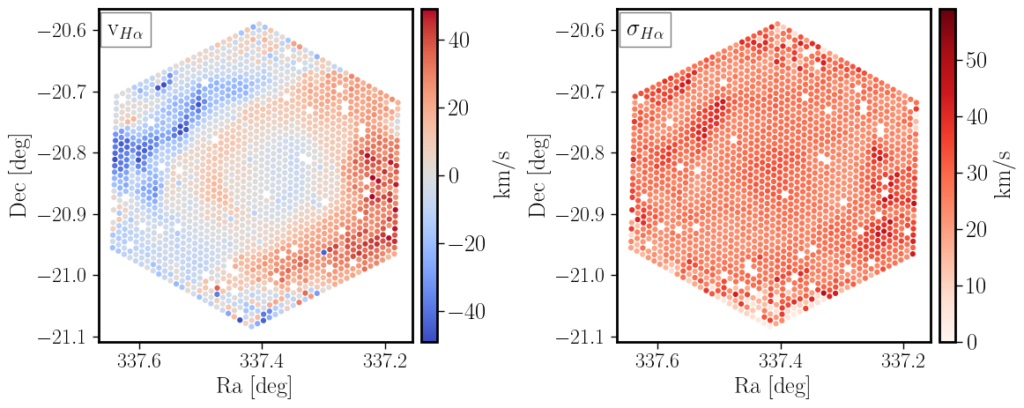
6. define generic helpers to plot any DAP column (line flux, equivalent width, velocity, stellar parameter, etc.) on the sky, and to compare the same quantity across different DAP measurement modes (non-parametric vs. PEK);
7. build Hα velocity and velocity-dispersion maps, reproducing the kinematic signature of the slowly expanding ionized shell of the Helix;
8. build a gallery of the brightest emission-line maps and a gallery of all good non-parametric lines, comparing strong and weak transitions on equal footing;
9. compute azimuthally averaged radial profiles of line fluxes and line ratios, both in absolute units and relative to Hβ, to study the ionization stratification of the nebula;
10. explore the stellar-continuum side of the DAP products: select fibers with measurable stellar continuum, plot diagnostic [Fe/H] [ /Fe] and T_eff log(g) distributions, and produce diagnostic plots such as Balmer-ratio comparisons and density-sensitive ratios versus line widths;
11. load the compact RSP template library used by the DAP, convert the per-fiber RSP coefficients into a long-format coefficient table, and reconstruct the full probability distribution functions of the stellar parameters for a given fiber, projected into the standard parameter planes (T_eff log(g), T_eff [ /Fe], [Fe/H] [ /Fe], [Fe/H] log(g)).

The RSP template files used by the DAP are distributed in a dedicated Google Drive folder (link); the notebook downloads automatically the templates required for the analysis based on the entries in the INFO extension of the DAP file.

---

4. Mosaic DAP tutorial

Notebook: lvm_dr20_Mosaic_DAP_tutorial.ipynb
Dataset: SDSS-V LVM DAP files for the M 33 (NGC 598) pointings released in DR20, using the experimental Milky Way foreground-subtracted products (LV_dap-rsp108-sn20-*.fits, EXPNUM = 5511 and 5512).

This notebook is the natural extension of the single-pointing DAP tutorial. It shows how to combine multiple DR20 DAP files into a single mosaic table, illustrating the workflow on the two M 33 pointings released in DR20 with the experimental Milky Way foreground-subtracted analysis (LV_dap* products). The unique id = EXPNUM.FIBERID key carried by every DAP table makes the stacking trivial: the resulting “mosaic” table contains exactly twice as many rows as a single pointing, and behaves transparently for all the visualization helpers introduced in the Helix tutorial.

The notebook teaches how to:

1. open and read several DR20 DAP products into a common astropy table by stacking the per-pointing tables;
2. build RGB emission-line maps that combine three tracers across the full mosaic, both for the strongest lines ([N II] 6583, Hα, [O III] 5007) and for the faintest diagnostic and auroral lines ([N II] 5755, Hε, [O III] 4363, [S III] 9531);
3. generate fiber-level BPT diagnostic diagrams on the mosaic, comparing log [O III]/Hβ against log [N II]/Hα, log [S II]/Hα, log [O II]/Hβ, and log [O I]/Hα with the demarcation curves used in the literature;
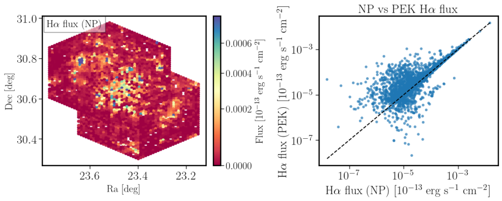
4. plot any DAP column on the sky for the full mosaic using the same generic helpers introduced in the single-pointing tutorial, and compare the same line measured with different DAP methods (non-parametric vs. PEK);
5. build Hα velocity and velocity-dispersion maps spanning the full mosaic;
6. explore the stellar side of the DAP products on a multi-pointing dataset, selecting fibers with measurable stellar continuum and inspecting the [Fe/H] [ /Fe] and T_eff log(g) distributions colored by distance from the mosaic center.

The same workflow applies to any future LVM mosaic. Although the example uses the M 33 LV_dap* products, switching to the corresponding standard dap-rsp108-sn20-*.fits files (with the Milky Way foreground preserved) only requires changing the file-selection variable at the top of the notebook.

---

5. DAP output-model generation

Notebook: lvm_dr20_generate_model_tutorial.ipynb
Dataset: SDSS-V LVM SFrame and DAP file for the Helix Nebula (DRPVER = 1.2.0, DAPVER = 1.2.0.251218, MJD = 60191, EXPNUM = 4297).

The DAP file delivers per-fiber measurements but does not, by itself, store the full spectral models. This tutorial shows how to reconstruct those models from the DAP outputs and the input SFrame, using the configuration parameters stored directly in the INFO extension of the DAP file. It is the notebook version of the gen_output_model.py workflow distributed with the LVM-DAP package, and produces a multi-plane FITS file containing every component of the spectral fit on the same wavelength grid as the data.

The notebook teaches how to:

1. locate the input lvmSFrame and the corresponding DAP file using sdss_access/sdss-tree, with a local fallback;
2. load the RSP template library used by the DAP, automatically downloading the required templates from the dedicated Google Drive when they are not in the local cache;
3. read the configuration parameters directly from the INFO extension of the DAP file, so that the model is generated with exactly the same setup that produced the released DAP measurements;
4. generate a multi-plane FITS output containing, for each science fiber: the original observed spectrum, the stellar model, the non-parametric gas model, the parametric gas model, the joint stellar+gas model, and the residual after subtracting the joint model;
5. plot the recovered model alongside the observed spectrum for an arbitrary fiber, to verify the quality of the spectral fit;
6. launch an interactive widget-based viewer (a modified version of the SFrame viewer described in tutorial 2) that displays, for any fiber selected on the sky map, the observed spectrum (black), the RSP stellar model (red), the parametric emission-line model (yellow), and the residuals (grey).

The output FITS file produced by this tutorial is the most direct way to inspect, fiber by fiber, the goodness-of-fit of the DAP analysis, and to use the modeled stellar continuum as a starting point for any custom emission-line analysis that goes beyond the lines already included in the DAP configuration.

---

6. DAP model-file reading tutorial

Notebook: lvm_dr20_read_model_tutorial.ipynb

Dataset: SDSS-V LVM DAP model file for the Helix Nebula (DRPVER = 1.2.0, DAPVER = 1.2.0.251218, MJD = 60191, EXPNUM = 4297).

This notebook complements the DAP reading and output-model generation tutorials by focusing on the direct inspection and visualization of the reconstructed spectral models stored in the DAP model-file product (dap-rsp108-sn20-EXPNUM.model.fits). The model file contains, for every analyzed science fiber, the observed spectrum together with the different spectral components reconstructed by the DAP analysis, including the stellar continuum model, the non-parametric and parametric gas models, the joint stellar+gas models, and the residual spectra.

The notebook teaches how to:

1. locate and open a DR20 DAP model file using sdss_access/sdss-tree, with a local-path fallback when needed;
2. inspect the FITS structure of the model file and recover the wavelength solution directly from the FITS header keywords;
3. identify the meaning of the nine model planes stored in the PRIMARY extension, including the observed spectrum, stellar-continuum model, gas-only spectra, non-parametric and parametric gas models, joint models, and residual products;
4. extract and visualize the reconstructed spectra for individual fibers across the full LVM wavelength range;
5. compare the observed spectrum with the stellar model, non-parametric gas model, parametric gas model, and joint model in selected spectral windows around strong nebular lines;
6. compute average spectra across the full field of view and compare the average reconstructed spectral components;
7. generate publication-style multi-panel spectral figures with inset zoom regions centered on strong and weak diagnostic emission lines;
8. inspect the residual spectra after subtracting the joint stellar+gas model as a diagnostic of the quality of the DAP fitting procedure.

The tutorial provides the most direct way to inspect the spectral decomposition performed by the LVM-DAP analysis and to understand how the released DAP measurements relate to the reconstructed spectral models stored in the companion model-file product. In nebular targets such as the Helix Nebula, the tutorial illustrates how the stellar and nebular contributions are separated fiber by fiber, and how the residual spectra can be used to assess the quality and limitations of the fits.

Example of the figures generated by the DAP model-file reading tutorial. Multi-component reconstruction of the average Helix Nebula spectrum derived from the DAP model file. The figure compares the observed spectrum, the reconstructed stellar continuum, the non-parametric and parametric gas models, and the final joint model over the full optical wavelength range. Insets centered on key diagnostic lines illustrate the quality of the reconstruction for both strong nebular transitions and faint auroral lines used for plasma diagnostics.

---

7. Quality-control bitmask tutorial

Notebook: lvm_dr20_drpall_dapall_qa_bitmask.ipynb
Dataset: DR20 LVM quality-control summary file (qcall-1.2.0-1.2.0.251218.fits)

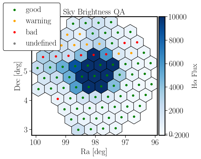
This notebook demonstrates how to read, decode, and use the DR20 LVM per-exposure quality-control bitmask. The qcall summary file provides, for each released exposure, a packed QA bitmask in which each metric is stored in a 2-bit field encoding one of four states: 00 = good, 01 = warning/minor issue, 10 = major issue, and 11 = not evaluated. The metrics covered include sky brightness, absolute and relative flux calibration, wavelength calibration, flatfield quality, sky-continuum and skyline subtraction, DAP fit quality, and visual inspection flags.

The notebook shows how to:

• open the qcall summary file and inspect its FITS structure and table contents;
• decode the qa_bitmask values into human-readable per-metric quality flags;
• extract individual QA parameters from the bitmask for a given exposure or for the full table;
• summarize the overall QA status into simple labels such as good, warning, or bad;
• join or cross-match the QA information with the drpall and dapall summary tables;
• filter exposures according to science-driven quality selections.

The notebook is intended as a practical guide for deciding which exposures are suitable for quantitative analysis and for understanding how individual QA metrics affect sample selection.

Getting the Tutorials

All notebooks listed above are distributed in the dedicated DR20 tutorials repository:

https://github.com/sdss/dr20_tutorials

Each tutorial includes its own list of Python dependencies; in general, all of them rely on numpy, matplotlib, and astropy. Tutorials 2 and 5 additionally use ipywidgets and ipympl for the interactive viewers, while tutorials 3, 4, and 5 use sdss-access, sdss-tree, and (optionally) gdown for retrieving the DAP files and RSP templates from the SAS and from the dedicated Google Drive folder.

For a description of the underlying data products, see the DR20 LVM page, the LVM Data Access page, and the LVM Data Analysis Pipeline page.