
For all observations in SDSS-V, there are bright limits that determine the sources that can be assigned to a fiber. There are two main considerations when determining these magnitude limits; at what magnitude all reductions become impossible (due to saturation of standards either directly or indirectly from contamination) and at what magnitude some reductions become impossible (e.g., at the faint end due to contamination of light from neighboring bright stars on the chip). For the former, this is the main consideration during Bright Time because we do not plan to observe stars at the very faint magnitude end of the dynamic range of the survey. For the dark time observing modes, the latter consideration is crucial because it is in these dark sky conditions we typically observe the faintest objects, as well as the objects requiring the best spectrophotometric accuracy. So, in certain regions of the sky this means objects brighter than some limit would typically be unobservable.
To avoid such a harsh limit, we developed an offsetting mode of operation. In this mode, we offset the fiber some predefined amount from the center of the object, such that the flux down the fiber will likely be fainter than the magnitude limit for that observation. Doing this accurately requires that typical shape of the Point Spread Function (PSF) must be well modeled. This was the subject of many commissioning tests, which are outlined in detail in Medan et al. (2025). Below we provide a brief summary of these tests and the fiber offset functions used throughout survey operations
Commissioning Tests
Initially, the PSF at larger angular separations was determined using archival eBOSS/BOSS data from SDSS DR16. For this analysis, we select all eBOSS/BOSS optical spectra that happen to lie within 90″ of a bright (VT < 12 mag) Tycho-2 star. We then compared the predicted flux based on SDSS photometry (CALIBFLUX) to the measured flux from the 1D spectra (SPECTROFLUX). Figure 1 shows the resulting median difference between these two values as a function of distance from the bright source. We fit functional forms that closely bound the data in three regions; core, transition and wings:
(1)
(2)
(3)
(4)
These functional forms were primarily used for bright star avoidance during the early stages of the survey.
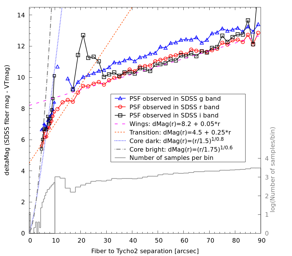
SPECTROFLUX–CALIBFLUX) and the magnitude of the nearby Tycho-2 source, versus angular distance to the Tycho-2 source.The above does not probe the flux loss at small offsets, where we will typically be placing fibers in this mode. To better measure the flux loss as a function of offset at small separations, we performed a series of commissioning observations during Bright and Dark time. In these observations, we intentionally offset the fiber from the center of a bright source by set amounts and compared the measured flux from the spectrum to the expected flux from photometric surveys. Figure 2 shows the result of such a test. To model the flux loss, we fit the data with a Moffat profile with radius equal to the circular fiber aperture, where we assume the fiber radius is 1” for APO and 0.665” for LCO. ere we show the prediction for the flux loss for a Moffat profile with two different FWHM values. We find that a value close to the typical seeing for that night produces the best fit.
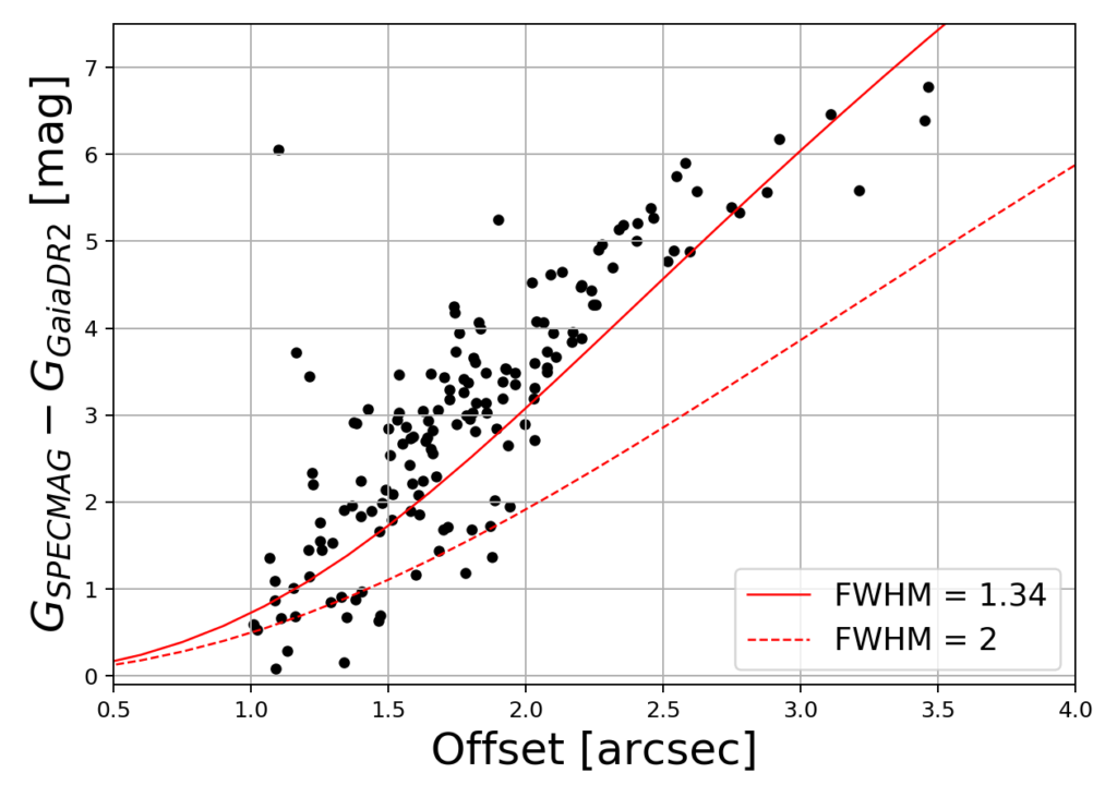
Because we precompute the offset when planning the survey before the actual observations (see robostrategy), we cannot incorporate the seeing at the time of observation to get the optimal FWHM for that night. Also, even within a night, there is significant scatter in the magnitude loss vs. fiber offset. So, we add another parameter to our offsetting method: the safety factor. This safety factor is a constant value added to the desired magnitude loss when calculating the offset of the fiber. With an appropriate safety factor, even if there is some scatter around the function all offset targets should still be dimmer than the magnitude limit for the observation.
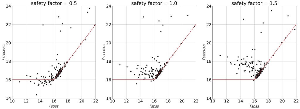
Figure 3 shows the r-band magnitude estimated from the spectrum versus true r-band magnitude for one of our commissioning tests. The different panels shows the result for different safety factors. We found a safety factor of 0.5 results in many targets having magnitudes brighter than the limit for the observation. At a safety factor of 1, almost all of the offset targets are fainter than the magnitude limit. When we increase the safety factor to 1.5, the offset targets become excessively faint, which could yield unusable results in this observing mode. Because this test was performed during dark time, where we are most concerned about contamination from on chip neighbors, we choose to use a safety factor of 1 for the offsetting in dark time. We also performed similar tests during bright time, and we concluded a safety factor of 0.5 was adequate.
Implementation of Offsets
The determination of a fiber offset is handled within coordio. Typically the functional form of the offset is described as a magnitude loss as a function of distance from the center of the target. Because we normally want an offset for a desired magnitude loss, we invert all formulations, where this is done analytically for eqs. 1-4 and done numerically via. linear interpolation for the Moffat profile.
For each target, the desired magnitude loss is the difference between the magnitude limit for the observation plus the safety factor (0.5 for Bright Time and 1 for Dark time) and the magnitude of the target. The offset that should give this desired magnitude loss is calculated for each regime (core, transition region and PSF wings) and the offset is the maximum value from these various functional forms. This process is repeated for each optical bandpass (g, r, i, z, BP, G, RP) with a magnitude limit for BOSS or each infrared bandpass (J, H, K) for APOGEE, and the final offset is the maximum value from the various photometric bands. Offsets are always applied in the positive Right Ascension direction. Ideally, we would always make the offset perpendicular to the parallactic angle to minimize chromatic effects associated with atmospheric differential refraction, but that would lead to unexpected collisions at observation time; choosing an offset in Right Ascension makes the offset more predictable while often being close to the desired direction. Additionally, offsets are prohibited for targets that are brighter than G=6 in Bright Time and G=13 magnitudes for Dark time for BOSS, and H=1 in all cases for APOGEE. So, such targets will not be observed during SDSS-V.
When reducing spectra of offset targets through the BOSS and APOGEE data reduction pipelines, offset targets are treated the same as nominal observations. This may have effects on the resulting spectrophotometry for the resulting spectra for offset targets, especially in the optical.
The definition of the core, transition region and PSF wings has changed throughout the survey. These changes historically coincide with a new series of the survey plan. Additionally, we have not always allowed offsetting during Bright and/or Dark time. The below table summarizes what functional forms were used and when offsetting was allowed during the different observational modes.
| Survey Plan Version | Core | Transition | Wings | Offsetting |
zeta (DR19) | Eqs. 1 & 2 | Eq. 3 | Eq. 4 | Bright time: NO Dark time: NO |
eta (DR20) | Moffat FWHM= 1.7′′ and β = 5 at APO Moffat FWHM= 1′′ and β = 2 at LCO | Eq. 3 | Eq. 4 | Bright time: YES Dark time: NO |
theta (DR20 & DR21) | Moffat FWHM= 0.5′′ and β = 1.6 at APO (Bright time) Moffat FWHM= 1.4′′ and β = 1.9 at APO (Dark time) Moffat FWHM= 0.8′′ and β = 1.7 at LCO (Bright time) Moffat FWHM= 1.1′′ and β = 1.8 at LCO (Dark time) | … | Eq. 4 | Bright time: YES Dark time: YES |